Statistics Manual [Draft]

by Andrey Akinshin

In this manual, I collect pragmatic statistical approaches that work well in practice.
Currently, this is a work-in-progress draft that selectively covers some topics; updates are coming.

Introduction

What we want from statistics is an easy-to-use tool that would nudge us toward asking the right questions and then straightforwardly guide us on how to design proper statistical procedures. What we often have is a bunch of vaguely described equations, arbitrarily chosen magical numbers as thresholds, and no clear understanding of what to do. Statistics is one of the most confusing, controversial, and depressing disciplines I know. So many different approaches, opinions, arguments, person-years of wasted time, and flawed peer-reviewed papers. The knowledge of rigorous proofs and asymptotic properties does not always help to approach real-life problems and find the optimal statistical method to use.

In this manual, I make my humble attempt to compose a guide for normal people who want to solve problems without being fooled by randomness whenever possible. The goals of the manual:

Provide simple and reliable statistical tools to get the job done
Explain ideas in a clear way for people without rich statistical experience and background
Form the right mindset for statistical thinking

The manual assumes some basic knowledge of statistics. I’m not going to spend much time explaining basic concepts. There are many good introductory books and I don’t see value repeating them in my own words for the sake of completeness. I limit the scope by brief definitions with relevant references, in which the reader may find more details. The target audience is people who already have some initial statistical experience and want to solve real-life problems.

Inspiration

I do not wish to judge how far my efforts coincide with those of other philosophers. Indeed, what I have written here makes no claim to novelty in detail, and the reason why I give no sources is that it is a matter of indifference to me whether the thoughts that I have had have been anticipated by someone else.¹

Most presented approaches are not new. Finding the “first appearance” of each particular idea is a challenging task.

Many times, I discovered myself in the following situation. I come up with a technique that naturally arises and addresses a particular real-life problem. Next, I start searching for this technique presented and explained in the literature. Occasionally, I find use cases of similar approaches without references or “formal” titles. They feel like common sense that does not require an “official” publication in which it’s explained. Who invented the idea and when did it happen are interesting questions from the historical perspective, but irrelevant from the pragmatic perspective.

When I have an explicit obvious reference to the original study, I provide it. Otherwise, I just present ideas as they are without attribution. I came up with usefulness of presented approaches on my own, but I’m standing on the shoulders of giants and was heavily inspired by works of other statisticians.

The content of this manual was significantly inspired by the following books that I revise from time to time:

Statistics Done Wrong · 2015 · Alex Reinhart
How to Lie with Statistics · 1982 · Darrell Huff
Probably Overthinking It · 2023 · Allen B. Downey

Introduction to Robust Estimation and Hypothesis Testing · 2021 · Rand R. Wilcox
Robust Statistics · 2009 · Peter J. Huber et al.
Robust Statistics · 2019 · Ricardo A Maronna et al.
Robust Statistics · 1986 · Frank R. Hampel et al.

The Fundamentals of Heavy Tails · 2022 · Jayakrishnan Nair et al.
Statistical Analysis of Extreme Values · 2001 · Rolf-Dieter Reiß et al.
Statistical Consequences of Fat Tails · 2020 · Nassim Nicholas Taleb

The Lady Tasting Tea · 2002 · David Salsburg
Statistical Methods for Research Workers · 1925 · Ronald A Fisher
Theoretical risks and tabular asterisks: Sir Karl, Sir Ronald, and the slow progress of soft ps... · 1978 · Paul E. Meehl
What If There Were No Significance Tests? · 1997 · Lisa L. Harlow
Statistical Rethinking · 2015 · Richard McElreath
Introduction to the New Statistics · 2024 · Geoff Cumming
Doing Bayesian Data Analysis · 2014 · John K. Kruschke
The Essential Guide to Effect Sizes · 2010 · Paul D. Ellis
Statistical Evidence · 1997 · Richard Royall

Some of my own works with new results:

Weighted quantile estimators
Trimmed Harrell-Davis quantile estimator based on the highest density interval of the given wid... · 2022
Quantile-respectful density estimation based on the Harrell-Davis quantile estimator · 2024
Quantile absolute deviation · 2022
Finite-sample bias-correction factors for the median absolute deviation based on the Harrell-Da... · 2022
Finite-sample Rousseeuw-Croux scale estimators · 2022

Statistical Flavors

The Neglect of Theoretical Statistics

Several reasons have contributed to the prolonged neglect into which the study of statistics, in its theoretical aspects, has fallen. ²

The “classic” theoretical statistics is a fascinating field of research with interesting findings and results. Unfortunately, most of these results are not so useful in practice.

This manual focuses on the pragmatic practical aspects. An approach works well in practice or it doesn’t work well in practice. All the other theoretical aspects are irrelevant. Simple Monte-Carlo simulations are more useful and insightful than rigorous proofs. We use theoretical aspects only when they contribute to better practical results.

From each statistical paradigm, we strive to extract the most useful and practical tools.

Parametric Statistics

Most classic statistical approaches are built around the normality assumption. However, the normal distribution is just a mathematical abstraction that does not exist in the real world in its pure form. It emerges in the limit case as a sum of random variables. If we have i.i.d. random variables $X_1, X_2, \ldots, X_n$, their sum $\left(X_1+X_2+\ldots+X_n\right)$ tends to be normal for $n\to\infty$ (under special conditions only). The convergence rate can be slow, so we should not expect the perfect normality for finite samples.

The normal distribution is an example of a parametric model. In parametric statistics, we have strict assumptions on the form of underlying distributions. Even small deviations from these assumptions may devalue the statistical inferences.

Nonparametric Statistics

While pure parametric methods are well-known and well-developed, they are not always applicable in practice. That is why the usage of parametric methods in their classic form is an unwise choice.

Fortunately, we have a handy alternative: the nonparametric statistic. This methodology rejects consider any parametric assumptions. While some implicit assumptions, like continuity or independence, still may be required, nonparametric statistics avoid considering any parametric models. Such methods are great when we have no prior knowledge about target distributions.

However, if the majority of collected data samples follow some patterns (which can be expressed in the form of parametric assumptions), nonparametric statistics do not look advantageous compared to the parametric methods because it is not capable of exploiting this prior knowledge to increase statistical efficiency.

Robust Statistics

Unlike parametric statistics, robust methods allow slight deviations from the declared parametric model. This gives reliable results even if some of the collected measurements do not meet our expectations. Unlike nonparametric statistics, robust methods do not fully reject parametric assumptions. This gives higher statistical efficiency compared to classic nonparametric statistics.

Recommended reading:
Introduction to Robust Estimation and Hypothesis Testing · 2021 · Rand R. Wilcox
Robust Statistics · 2009 · Peter J. Huber et al.
Robust Statistics · 2019 · Ricardo A Maronna et al.
Robust Statistics · 1986 · Frank R. Hampel et al.

Unfortunately, classic robust statistics have issues in the case of huge deviations from the assumptions. Usually, robust statistical methods are not capable of handling extreme corner cases, which also can arise in practice.

Defensive Statistics

Defensive statistics tries to get benefits from all the above methodologies. Like parametric statistics, it accepts the fact that the majority of the collected data samples may follow specific patterns. If we express these patterns in the form of assumptions, we can significantly increase statistical efficiency in most cases. Like robust statistics, it accepts small deviations from the assumptions and continues to provide reliable results in the corresponding cases. Like nonparametric statistics, it accepts huge deviations from the assumptions and tries to continue to provide reasonable results even in the cases of malformed or corrupted data. However, unlike nonparametric statistics, it doesn’t stop acknowledging the original assumptions. Therefore, defensive statistics ensures not only high reliability but also high efficiency in the majority of cases.

Pragmatic Statistics

Let me make an attempt to speculate on the principles that should form the foundation of the Pragmatic statistics approach.

Pragmatic statistics is useful statistics.
We use statistics to actually get things done and solve actual problems. We do not use statistics to make our work more “scientific” or just because everyone else does it.
Pragmatic statistics is goal-driven statistics.
We always clearly define the goals we want to achieve and the problems we want to solve. We do not apply statistics to just check out how the data looks like and we do not draw conclusions from exploratory research without additional confirmatory research.
Pragmatic statistics is verifiable statistics.
Based on the clearly defined goals, we should build a verification framework that allows checking if the considered statistical approaches match the goals. Therefore, choosing the proper research design among several options should be a mechanical process.
Pragmatic statistics is efficient statistics.
We aim to get the maximum statistical efficiency. We understand that the data collection is not free and we want to fully utilize the information we obtain.
Pragmatic statistics is eclectic statistics.
We do not ban statistical methods just because they are “bad.” We are ready to use any combination of methods from different statistical paradigms while they solve the problem.
Pragmatic statistics is estimation statistics.
We focus on practical significance instead of statistical significance. We never ask, “Is there an effect?”; we always assume that an effect always exists and our primary question is about the magnitude of the effect.
Pragmatic statistics is robust statistics.
We are ready to handle extreme outliers in our data and heavy-tailed distributions in our models.
Pragmatic statistics is nonparametric statistics.
While we try to utilize existing parametric assumptions to increase efficiency, we embrace deviations from the given parametric model and adjust the approaches for the nonparametric case.
Pragmatic statistics is defensive statistics.
We aim to support all the corner cases. While robust and nonparametric approaches help us to handle moderate deviations from the model, severe assumption violations should not lead to misleading or incorrect inference.
Pragmatic statistics is weighted statistics.
We do not treat all the obtained measurements equally. Instead, we try to extend the model with weight coefficients that reflect the representativeness of the measurements.

Pragmatic Summary Estimators

In this section, we suggest pragmatic estimators to summarize a single sample $\mathbf{x} = (x_1, x_2, \ldots, x_n)$ or compare it to a sample $\mathbf{y} = (y_1, y_2, \ldots, y_m)$. First, we briefly introduce them and next review one by one.

Center (Average, Location, Central Tendency)

When people encounter a large sample of values, they naturally feel a desire to “compress” it into a single “average” number. The most default choice is the The Arithmetic Mean. This measure is not robust: a single extreme value can distort the result. Another alternative is The Sample Median. It’s highly robust, but not efficient (has lower precision): the median estimations are more dispersed than the mean ones under normality. For a better trade-off between robustness and efficiency, we suggest the Hodges-Lehmann Estimator:

$$ \mu_x = \operatorname{HL}(\mathbf{x}) = \underset{1 \leq i \leq j \leq n}{\operatorname{Median}} \left(\dfrac{x_i + x_j}{2} \right) $$

For simplicity, we refer the Hodges-Lehmann estimator as “center” and denote by $\mu$ (do not confuse with the arithmetic mean). In discussions of the normal distribution, we present notation separately.

The Hodges-Lehmann estimator has Gaussian efficiency of $\approx 96\%$. It’s also known as pseudomedian.

Spread (Dispersion, Measure of Variability)

The most popular measure of dispersion is the standard deviation. In the perfectly normal world, it feels natural to use it as a universal measure of dispersion. In the pragmatic statistics, we strive to avoid the standard deviation whenever possible. If the data doesn’t follow the normal distribution, its usage is meaningless and misleading. Moreover, the concept of the standard deviation itself is confusing for people. The standard deviation is essentially a parameter $\sigma$ of the normal distribution defined as $f(x) = e^{-\frac{(x-\mu)^2}{2\sigma^2}} / \sqrt{2\pi\sigma^2}$. Not so many people can recall this equation or provide the definition of the standard deviation. Correct interpretation of its values is challenging by nature since the 68–95–99.7 rule doesn’t work for many real data sets. People who encounter the standard deviation in statistical reports often don’t understand what it means and how to use it.

As a more intuitive and pragmatic alternative, we use the Shamos Estimator:

$$ \sigma_x = \operatorname{Shamos}(\mathbf{x}) = \underset{i < j}{\operatorname{Median}} (|x_i - x_j|), $$

For simplicity, we refer the Shamos estimator as “spread” and denote by $\sigma$ (do not confuse with the standard deviation). In discussions of the normal distribution, we present notation separately.

Such definition is easier to understand: it’s the median absolute difference between pairs of values. If the normality assumption is met, the Shamos estimator can be scaled to be consistent with the standard deviation under normality with Gaussian efficiency of $\approx 86\%$. Its breakdown point is $\approx 29\%$.

Shift (absolute shift, location shift, absolute location difference, Hodges-Lehmann shift estimator):

$$ \mu_{xy} = \underset{1 \leq i \leq n,\,\, 1 \leq j \leq m}{\operatorname{Median}} \left(x_i - y_j \right) $$

Ratio:

$$ \rho_{xy} = \underset{1 \leq i \leq n,\,\, 1 \leq j \leq m}{\operatorname{Median}} \left( \dfrac{x_i}{y_j} \right) $$

Disparity (Difference Effect Size, Normalized Shift):

$$ \psi_{xy} = \dfrac{\mu_{xy}}{\sigma_{xy}},\quad \psi_{*xy} = \dfrac{\mu_{xy}}{\sigma_{x}},\quad \psi_{xy*} = \dfrac{\mu_{xy}}{\sigma_{y}},\quad \sigma_{xy} = \dfrac{n\sigma_x + m\sigma_y}{n + m} $$

Center

As a measure of centeral tendency (location, average), we use Hodges-Lehmann Estimator:

$$ \mu_x = \operatorname{HL}(\mathbf{x}) = \underset{1 \leq i \leq j \leq n}{\operatorname{Median}} \left(\dfrac{x_i + x_j}{2} \right) $$

Let’s compare it with other classic measures. The Arithmetic Mean $\overline{\mathbf{x}} = (x_1 + x_2 + \ldots + x_n)/n$ is the “default” synonym for the average. Works well for normal data but is not robust. In the case of statistical artifacts like outliers, multimodality, asymmetry, discretization, the mean loses statistical efficiency and starts to behave unreliably. A single extreme value can distort the mean value and make it meaningless. The mean of (1, 2, 3, 4, 5, 6, 273) is 42. In 1986, the average starting annual salary of geography graduates from the University of North Carolina was \$250 000 thanks to Michael Jordan who made over \$700 000 in the NBA. The mean is too fragile to be used with real data.

The Sample Median is the “second default” synonym for the average. The median addresses some disadvantages of the mean and feels like a more reasonable metric to use. The median of (1, 2, 3, 4, 5, 6, 273) is 4. The median American has a net worth of \$192 900 while the Mean American has \$1 063 700. . The median has a breakdown point of 50%. This means that we can corrupt up to 50% of the data, but the median will remain the same. Exceptional robustness comes with a price of lower statistical efficiency. Efficiency describes the size of random errors. The better the efficiency, the more precise the measurements. There is a trade-off between robustness and efficiency. Under the perfect normal distribution, the mean is the best average estimator. It has an efficiency of 100%, but its breakdown point is 0%. The breakdown point of the median is 50%, but its efficiency is only 64%.

The Hodges-Lehmann average $\operatorname{HL}$ provides a better trade-off. Under normality, $\operatorname{HL}$ has a breakdown point of 29% and an efficiency of 96%. Such a level of robustness is good enough in practice. If more than 29% of the data are outliers, it’s probably a multimodal distribution, which we should handle separately. We don’t need higher robustness.

Here are the comparisons of relative efficiency to the mean under the normal and uniform distributions:

Distribution	Median	Hodges-Lehmann
Gaussian	≈64%	≈96%
Uniform	≈34%	≈97%

If we take random samples from the uniform distribution of size 10, and measure the mean, the median, and the Hodges-Lehmann average for each sample, we will get the following sampling distributions:

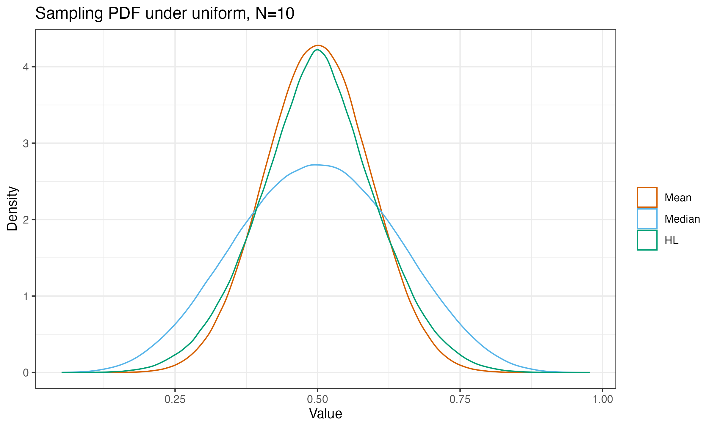
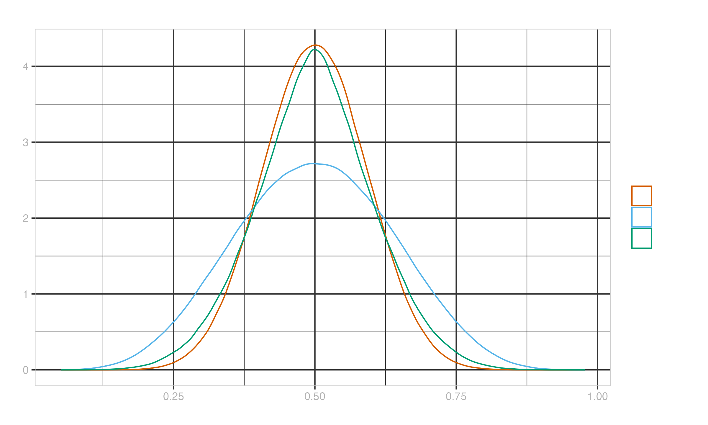
Note that the curves of the mean and $\operatorname{HL}$ are close to each other, while the median curve is more dispersed. We can consider such a difference from a more practical perspective. Let’s say we spend \$100 to gather a sample of the given size. If we switch from the mean to another estimator, we have to adjust the sample size to achieve the same precision. That’s how it affects the budget:

Distribution	Median	Hodges-Lehmann
Gaussian	\$156	\$104
Uniform	\$294	\$103

The Hodges-Lehmann average is a safe rule-of-thumb for initial insights into the data. It’s also a pragmatic choice of the measure of central tendency or location for further statistical procedures.

Spread

As a measure of dispersion, we use the Shamos Estimator:

$$ \sigma_x = \operatorname{Shamos}(\mathbf{x}) = \underset{i < j}{\operatorname{Median}} (|x_i - x_j|), $$

The asymptotic Gaussian efficiency is of $\approx 86\%$; the asymptotic breakdown point is of $\approx 29\%$. The finite-sample consistency factor and efficiency values can be found in park2020. In rousseeuw1993, it is claimed that the Rousseeuw-Croux estimator is a good alternative with much higher breakdown point of $50\%$ and slightly decorated statistical efficiency (the asymptotic value is of $\approx 82\%$). However, for small samples the efficiency gap is huge, so I prefer the Shamos estimator.