Caveats of using the median absolute deviation

The median absolute deviation is a measure of dispersion which can be used as a robust alternative to the standard deviation. It works great for slight deviations from normality (e.g., for contaminated normal distributions or slightly skewed unimodal distributions). Unfortunately, if we apply it to distributions with huge deviations from normality, we may experience a lot of troubles. In this post, I discuss some of the most important caveats which we should keep in mind if we use the median absolute deviation.

Preprint announcement: 'Finite-sample bias-correction factors for the median absolute deviation based on the Harrell-Davis quantile estimator and its trimmed modification'

I have just published a preprint of a paper ‘Finite-sample bias-correction factors for the median absolute deviation based on the Harrell-Davis quantile estimator and its trimmed modification’. It’s based on a series of my research notes that I have been writing since February 2021.

The paper preprint is available on arXiv: arXiv:2207.12005 [stat.ME]. The paper source code is available on GitHub: AndreyAkinshin/paper-mad-factors. You can cite it as follows:

• Andrey Akinshin (2022) “Finite-sample bias-correction factors for the median absolute deviation based on the Harrell-Davis quantile estimator and its trimmed modification,” arXiv:2207.12005

Abstract:

The median absolute deviation is a widely used robust measure of statistical dispersion. Using a scale constant, we can use it as an asymptotically consistent estimator for the standard deviation under normality. For finite samples, the scale constant should be corrected in order to obtain an unbiased estimator. The bias-correction factor depends on the sample size and the median estimator. When we use the traditional sample median, the factor values are well known, but this approach does not provide optimal statistical efficiency. In this paper, we present the bias-correction factors for the median absolute deviation based on the Harrell-Davis quantile estimator and its trimmed modification which allow us to achieve better statistical efficiency of the standard deviation estimations. The obtained estimators are especially useful for samples with a small number of elements.

Challenges of change point detection in CI performance data

Change point detection is a popular task in various disciplines. There are many algorithms that solve this problem. For example, in truong2020, the authors presented a classification of different approaches and discussed 35 algorithms. However, not all the algorithms fit all the situations.

In this post, we consider the problem of change point detection in time series based on software performance measurements obtained from a continuous integration (CI) server. Examples of data sources are CI builds, unit tests, benchmarks, performance tests, and so on. We would like to automatically find performance degradations in such time series. Unfortunately, most of the available algorithms do not provide decent solutions for this problem. In this post, I discuss some challenges that arise when we are looking for change points in CI performance data.

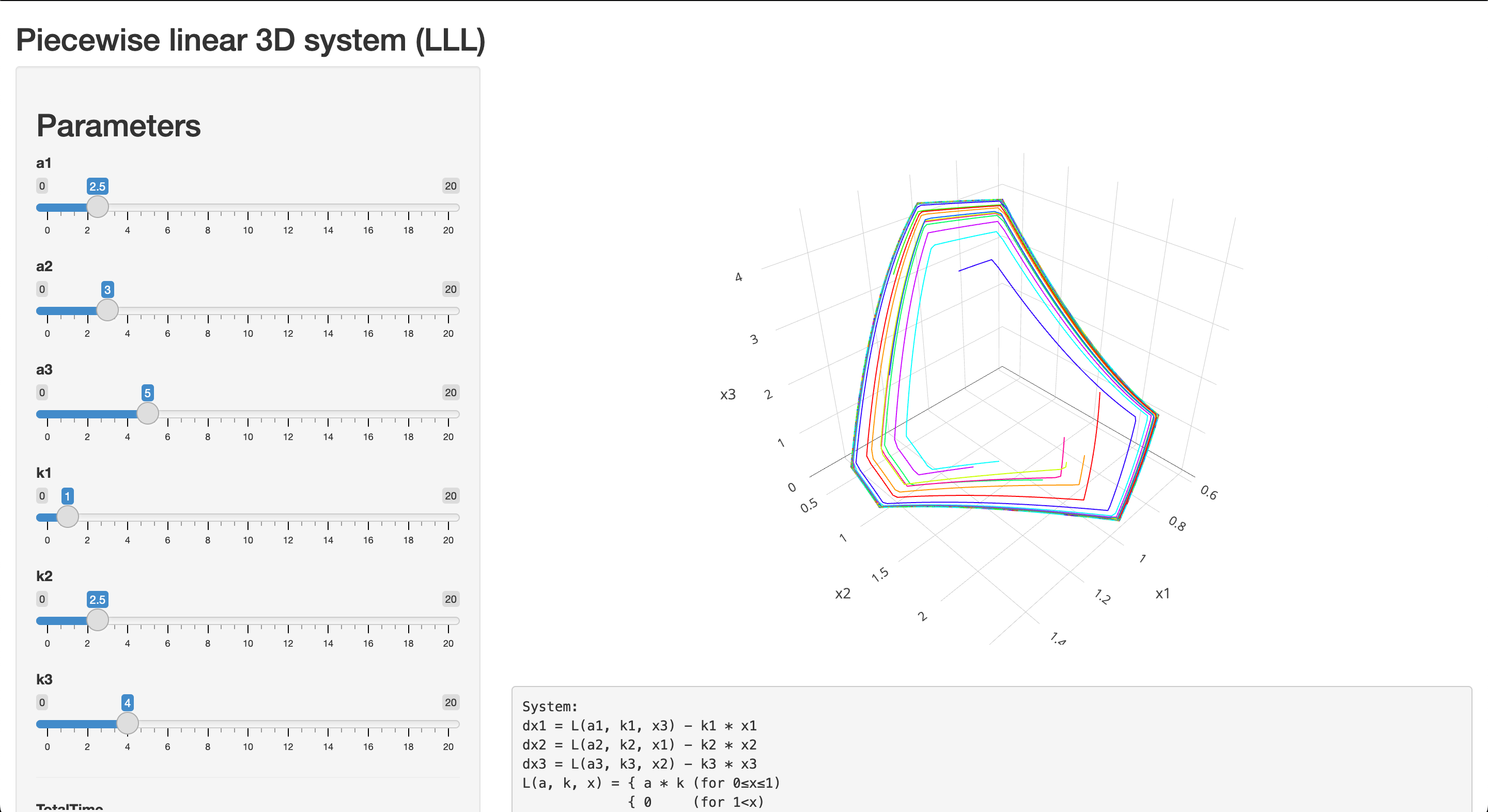
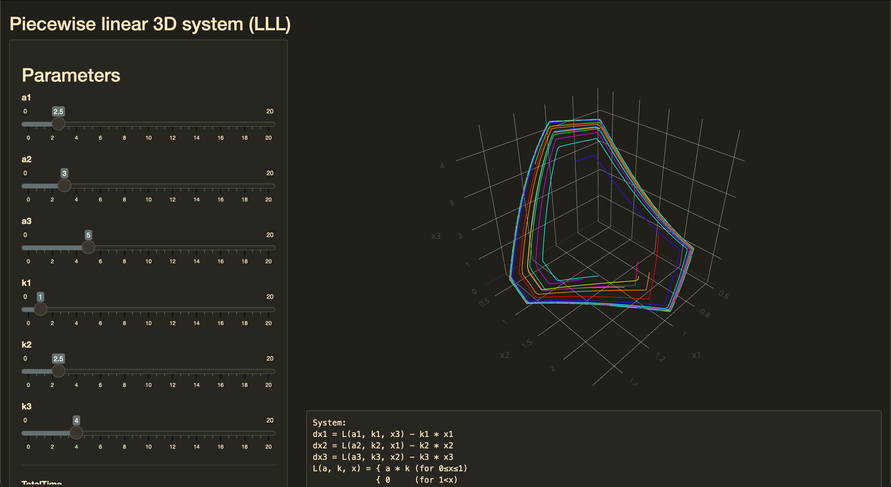
Dynamical System Case Study 2 (Piecewise linear LLL-system)

We consider the following dynamical system:

where $L$ is a piecewise linear function:

In this case study, we build a Shiny application that draws 3D phase portraits of this system for various sets of input parameters.

Degenerate point of dispersion estimators

Recently, I have been working on searching for a robust statistical dispersion estimator that doesn’t become zero on samples with a huge number of tied values. I have already created a few of such estimators like the middle non-zero quantile absolute deviation (part 1, part 2) and the untied quantile absolute deviation. Having several options to compare, we need a proper metric that allows us to perform such a comparison. Similar to the breakdown point (that is used to describe estimator robustness), we could introduce the degenerate point that describes the resistance of a dispersion estimator to the tied values. In this post, I will briefly describe this concept.

Untied quantile absolute deviation

In the previous posts, I tried to adapt the concept of the quantile absolute deviation to samples with tied values so that this measure of dispersion never becomes zero for nondegenerate ranges. My previous attempt was the middle non-zero quantile absolute deviation (modification 1, modification 2). However, I’m not completely satisfied with the behavior of this metric. In this post, I want to consider another way to work around the problem with tied values.

Middle non-zero quantile absolute deviation, Part 2

In one of the previous posts, I described the idea of the middle non-zero quantile absolute deviation. It’s defined as follows:

where $\mathbf{1}$ is the indicator function

and $\operatorname{QAD}$ is the quantile absolute deviation

The $\operatorname{MNZQAD}$ approach tries to work around a problem with tied values. While it works well in the generic case, there are some corner cases where the suggested metric behaves poorly. In this post, we discuss this problem and how to solve it.

The expected number of takes from a discrete distribution before observing the given element

Let’s consider a discrete distribution $X$ defined by its probability mass function $p_X(x)$. We randomly take elements from $X$ until we observe the given element $x_0$. What’s the expected number of takes in this process?

This classic statistical problem could be solved in various ways. I would like to share one of my favorite approaches that involves the derivative of the series $\sum_{n=0}^\infty x^n$.