Unbiased median absolute deviation for n=2

I already covered the topic of the unbiased median deviation based on the traditional sample median, the Harrell-Davis quantile estimator, and the trimmed Harrell-Davis quantile estimator. In all the posts, the values of bias-correction factors were evaluated using the Monte-Carlo simulation. In this post, we calculate the exact value of the bias-correction factor for two-element samples.

Weighted trimmed Harrell-Davis quantile estimator

In this post, I combine ideas from two of my previous posts:

• Trimmed Harrell-Davis quantile estimator: quantile estimator that provides an optimal trade-off between statistical efficiency and robustness
• Weighted quantile estimators: a general scheme that allows building weighted quantile estimators. Could be used for quantile exponential smoothing and dispersion exponential smoothing.

Thus, we are going to build a weighted version of the trimmed Harrell-Davis quantile estimator based on the highest density interval of the given width.

Minimum meaningful statistical level for the Mann–Whitney U test

The Mann–Whitney U test is one of the most popular nonparametric null hypothesis significance tests. However, like any statistical test, it has limitations. We should always carefully match them with our business requirements. In this post, we discuss how to properly choose the statistical level for the Mann–Whitney U test on small samples.

Let’s say we want to compare two samples $x = \{ x_1, x_2, \ldots, x_n \}$ and $y = \{ y_1, y_2, \ldots, y_m \}$ using the one-sided Mann–Whitney U test. Sometimes, we don’t have an opportunity to gather enough data and we have to work with small samples. Imagine that the size of both samples is six: $n=m=6$. We want to set the statistical level $\alpha$ to $0.001$ (because we really don’t want to get false-positive results). Is it a valid requirement? In fact, the minimum p-value we can observe with $n=m=6$ is $\approx 0.001082$. Thus, with $\alpha = 0.001$, it’s impossible to get a positive result. Meanwhile, everything is correct from the technical point of view: since we can’t get any positive results, the false positive rate is exactly zero which is less than $0.001$. However, it’s definitely not something that we want: with this setup the test becomes useless because it always provides negative results regardless of the input data.

This brings an important question: what is the minimum meaningful statistical level that we can require for the one-sided Mann–Whitney U test knowing the sample sizes?

Fence-based outlier detectors, Part 2

In the previous post, I discussed different fence-based outlier detectors. In this post, I show some examples of these detectors with different parameters.

Fence-based outlier detectors, Part 1

In previous posts, I discussed properties of Tukey’s fences and asymmetric decile-based outlier detector (Part 1, Part 2). In this post, I discuss the generalization of fence-based outlier detectors.

Publication announcement: 'Trimmed Harrell-Davis quantile estimator based on the highest density interval of the given width'

Since the beginning of previous year, I have been working on building a quantile estimator that provides an optimal trade-off between statistical efficiency and robustness. At the end of the year, I published the corresponding preprint where I presented a description of such an estimator: arXiv:2111.11776 [stat.ME]. The paper source code is available on GitHub: AndreyAkinshin/paper-thdqe.

Finally, the paper was published in Communications in Statistics - Simulation and Computation. You can cite it as follows:

• Andrey Akinshin (2022) Trimmed Harrell-Davis quantile estimator based on the highest density interval of the given width, Communications in Statistics - Simulation and Computation, DOI: 10.1080/03610918.2022.2050396

Asymmetric decile-based outlier detector, Part 2

In the previous post, I suggested an asymmetric decile-based outlier detector as an alternative to Tukey’s fences. In this post, we run some numerical simulations to check out the suggested outlier detector in action.

Asymmetric decile-based outlier detector, Part 1

In the previous post, I covered some problems with the outlier detector based on Tukey fences. Mainly, I discussed the probability of observing outliers using Tukey’s fences with different factors under different distributions. However, it’s not the only problem with this approach.

Since Tukey’s fences are based on quartiles, under multimodal distributions, we could get a situation when 50% of all sample elements are marked as outliers. Also, Tukey’s fences are designed for symmetric distributions, so we could get strange results with asymmetric distributions.

In this post, I want to suggest an asymmetric outlier detector based on deciles which mitigates this problem.

Probability of observing outliers using Tukey's fences

Tukey’s fences is one of the most popular simple outlier detectors for one-dimensional number arrays. This approach assumes that for a given sample, we calculate first and third quartiles ($Q_1$ and $Q_3$), and mark all the sample elements outside the interval

as outliers. Typical recommendation for $k$ is $1.5$ for “regular” outliers and $3.0$ for “far outliers”. Here is a box plot example for a sample taken from the standard normal distributions (sample size is $1000$):

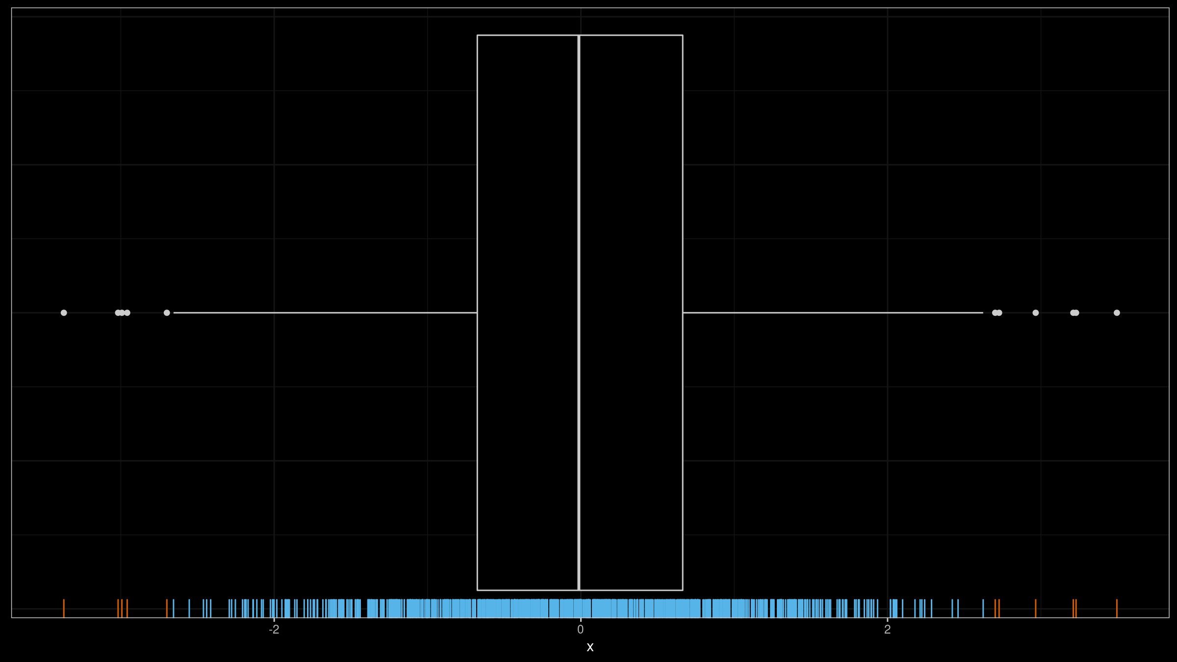
As we can see, 11 elements were marked as outliers (shown as dots). Is it an expected result or not? The answer depends on your goals. There is no single definition of an outlier. In fact, the chosen outlier detector provides a unique outlier definition.

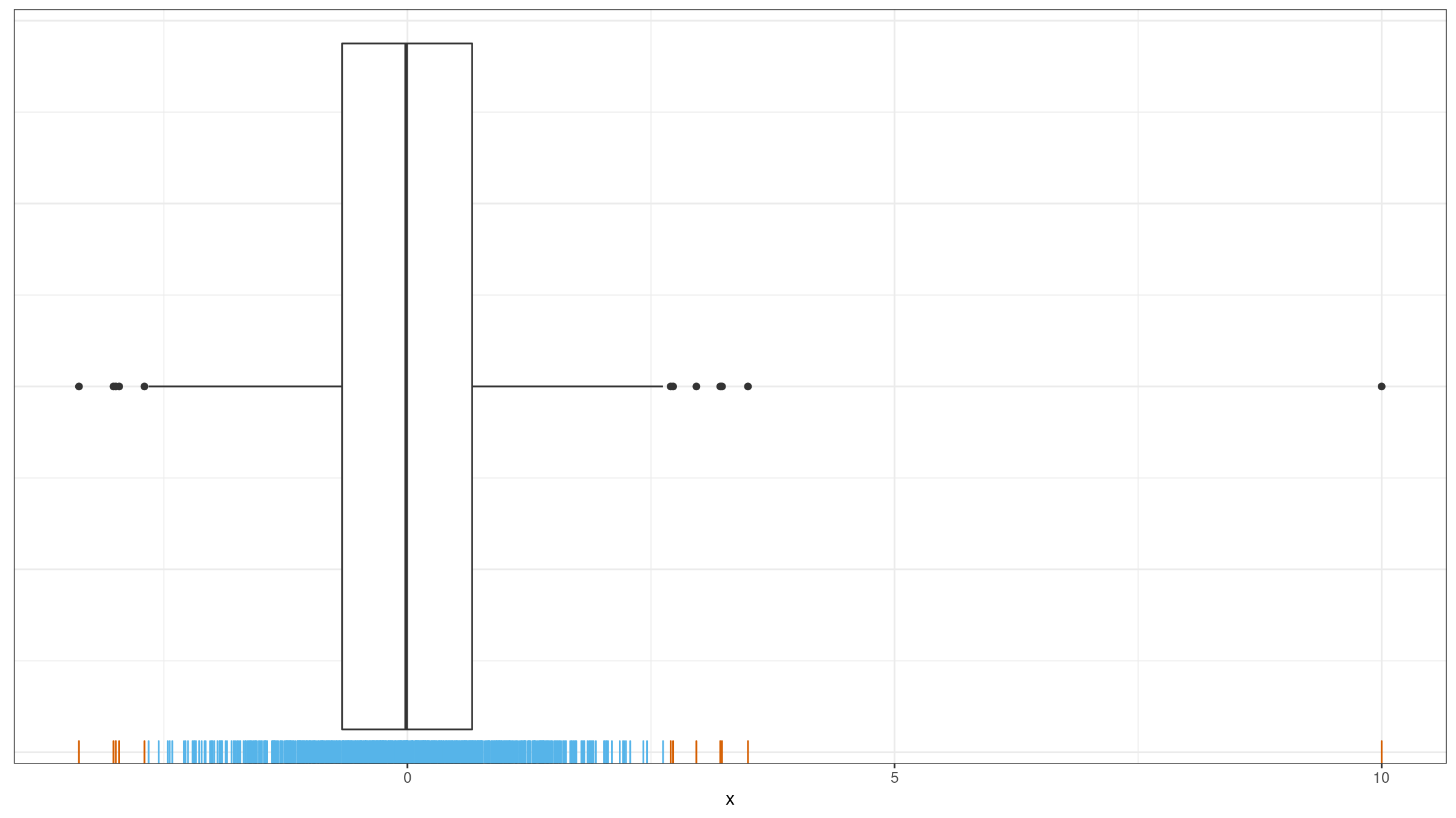
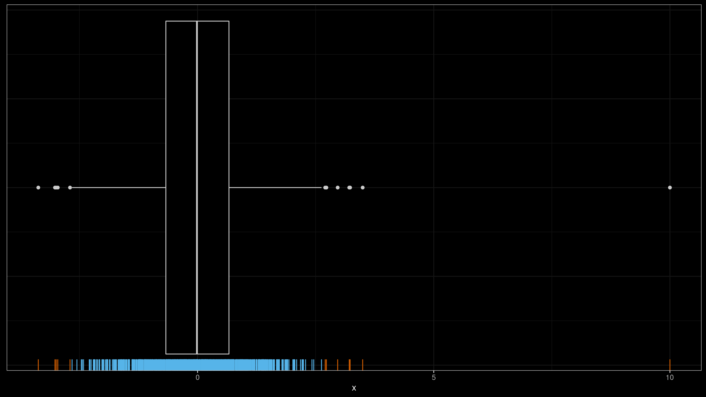
In my applications, I typically consider outliers as rare events that should be investigated. When I detect too many outliers, all such reports become useless noise. For example, on the above image, I wouldn’t treat any of the sample elements as outliers. However, If we add $10.0$ to this sample, this element is an obvious outlier (which will be the only one):

Thus, an important property of an outlier detector is the “false positive rate”: the percentage of samples with detected outliers which I wouldn’t treat as outliers. In this post, I perform numerical simulations that show the probability of observing outliers using Tukey’s fences with different $k$ values.