Matching quantile sets using likelihood based on the binomial coefficients

Let’s say we have a distribution $X$ that is given by its $s$-quantile values:

where $Q_X$ is the quantile function of $X$, $p_j = j / s$.

We also have a sample $y = \{y_1, y_2, \ldots, y_n \}$ that is given by its $s$-quantile estimations:

where $Q_y$ is the quantile estimation function for sample $y$. We also assume that $q_{y_0} = \min(y)$, $q_{y_s} = \max(y)$.

We want to know the likelihood of “$y$ is drawn from $X$”. In this post, I want to suggest a nice way to do this using the binomial coefficients.

Ratio function vs. ratio distribution

Let’s say we have two distributions $X$ and $Y$. In the previous post, we discussed how to express the “absolute difference” between them using the shift function and the shift distribution. Now let’s discuss how to express the “relative difference” between them. This abstract term also could be expressed in various ways. My favorite approach is to build the ratio function. In order to do this, for each quantile $p$, we should calculate $Q_Y(p)/Q_X(p)$ where $Q$ is the quantile function. However, some people prefer using the ratio distribution $Y/X$. While both approaches may provide similar results for narrow positive non-overlapping distributions, they are not equivalent in the general case. In this post, we briefly consider examples of both approaches.

Shift function vs. shift distribution

Let’s say we have two distributions $X$ and $Y$, and we want to express the “absolute difference” between them. This abstract term could be expressed in various ways. My favorite approach is to build the Doksum’s shift function. In order to do this, for each quantile $p$, we should calculate $Q_Y(p)-Q_X(p)$ where $Q$ is the quantile function. However, some people prefer using the shift distribution $Y-X$. While both approaches may provide similar results for narrow non-overlapping distributions, they are not equivalent in the general case. In this post, we briefly consider examples of both approaches.

Preprint announcement: 'Trimmed Harrell-Davis quantile estimator based on the highest density interval of the given width'

Update: the final paper was published in Communications in Statistics - Simulation and Computation (DOI: 10.1080/03610918.2022.2050396).

Since the beginning of this year, I have been working on building a quantile estimator that provides an optimal trade-off between statistical efficiency and robustness. Finally, I have built such an estimator. A paper preprint is available on arXiv: arXiv:2111.11776 [stat.ME]. The paper source code is available on GitHub: AndreyAkinshin/paper-thdqe. You can cite it as follows:

• Andrey Akinshin (2021) Trimmed Harrell-Davis quantile estimator based on the highest density interval of the given width, arXiv:2111.11776

Non-normal median sampling distribution

Let’s consider the classic sample median. If a sample is sorted and the number of sample elements is odd, the median is the middle element. In the case of an even number of sample elements, the median is an arithmetic average of the two middle elements.

Now let’s say we randomly take many samples from the same distribution and calculate the median for each of them. Next, we build a sampling distribution based on these median values. There is a well-known fact that this distribution is asymptotically normal with mean $M$ and variance $1/(4nf^2(M))$, where $n$ is the number of elements in samples, $f$ is the probability density function of the original distribution, and $M$ is the true median of the original distribution.

Unfortunately, if we try to build such sampling distributions in practice, we may see that they are not always normal. There are some corner cases that prevent us from using the normal model in general. If you implement general routines that analyze the median behavior, you should keep such cases in mind. In this post, we briefly talk about some of these cases.

Misleading kurtosis

I already discussed misleadingness of such metrics like standard deviation and skewness. It’s time to discuss misleadingness of the measure of tailedness: kurtosis (which, sometimes, could be incorrectly interpreted as a measure of peakedness). Typically, the concept of kurtosis is explained with the help of images like this:

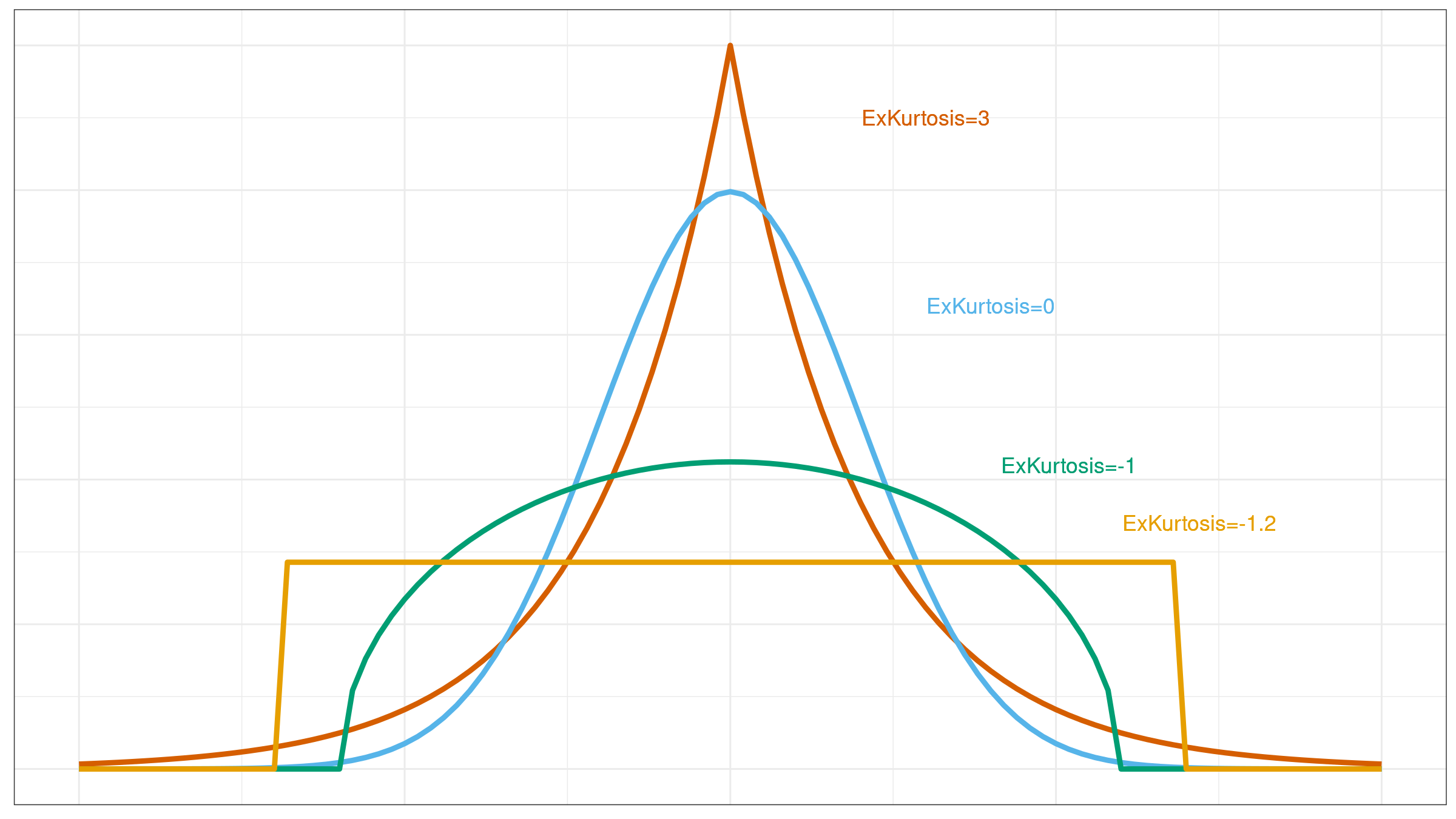
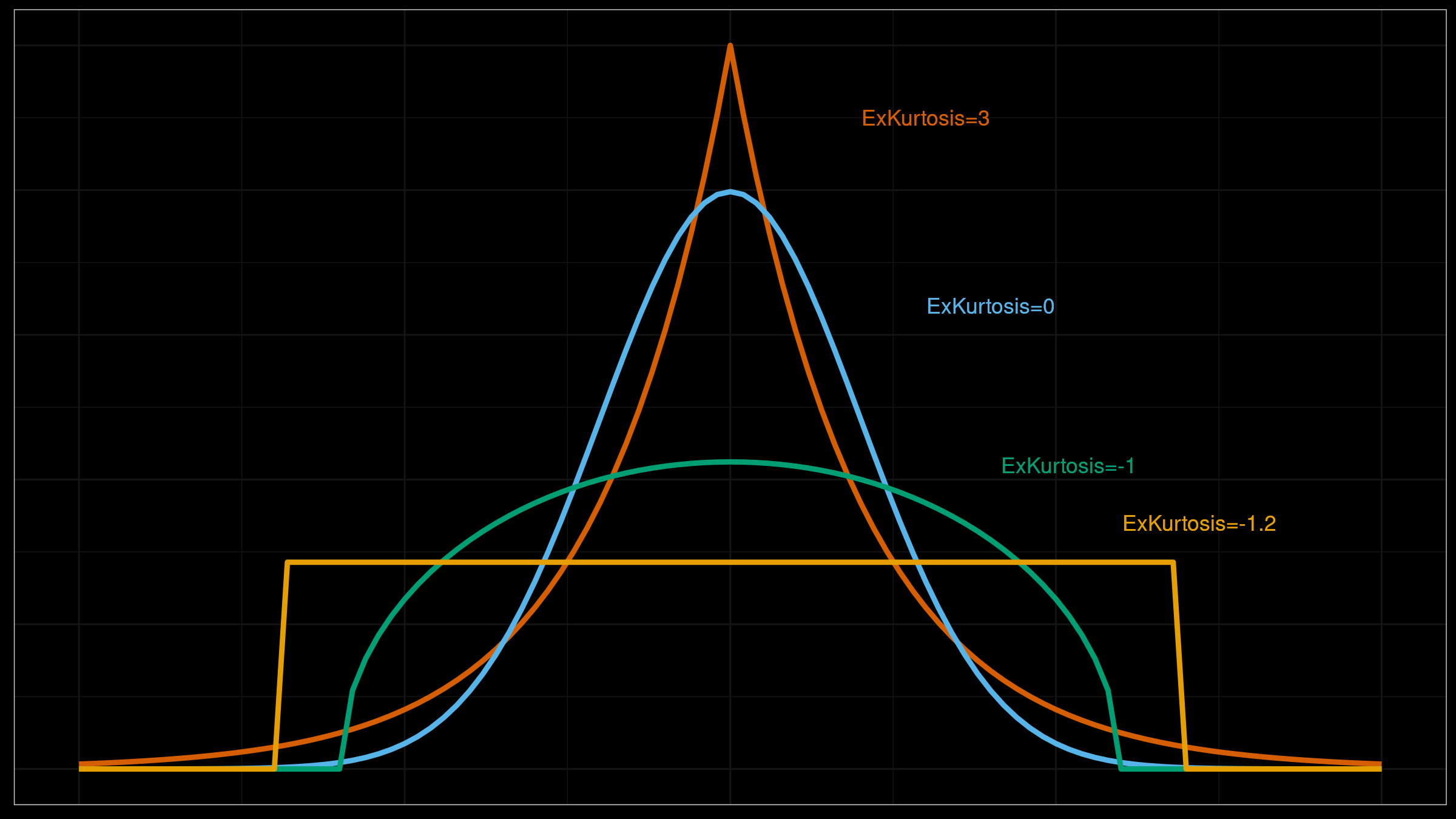
Unfortunately, the raw kurtosis value may provide wrong insights about distribution properties. In this post, we briefly discuss the sources of its misleadingness:

• There are multiple definitions of kurtosis. The most significant confusion arises between “kurtosis” and “excess kurtosis,” but there are other definitions of this measure.
• Kurtosis may work fine for unimodal distributions, but it performs not so clear for multimodal distributions.
• The classic definition of kurtosis is not robust: it could be easily spoiled by extreme outliers.

Misleading skewness

Skewness is a commonly used measure of the asymmetry of the probability distributions. A typical skewness interpretation comes down to an image like this:

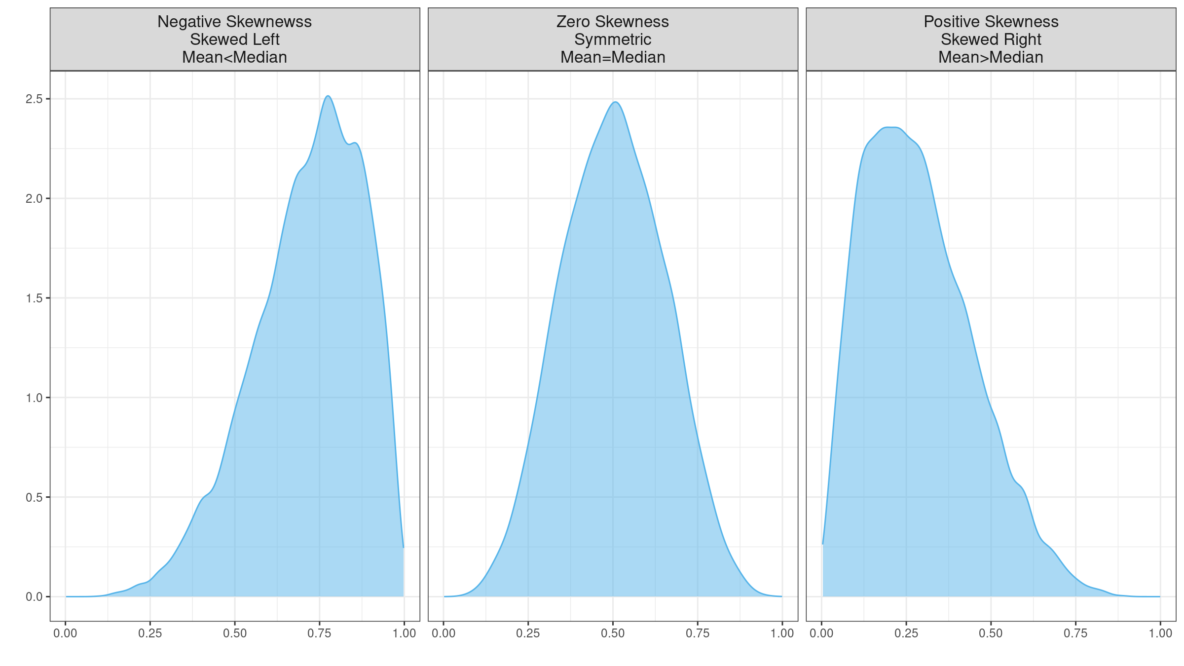
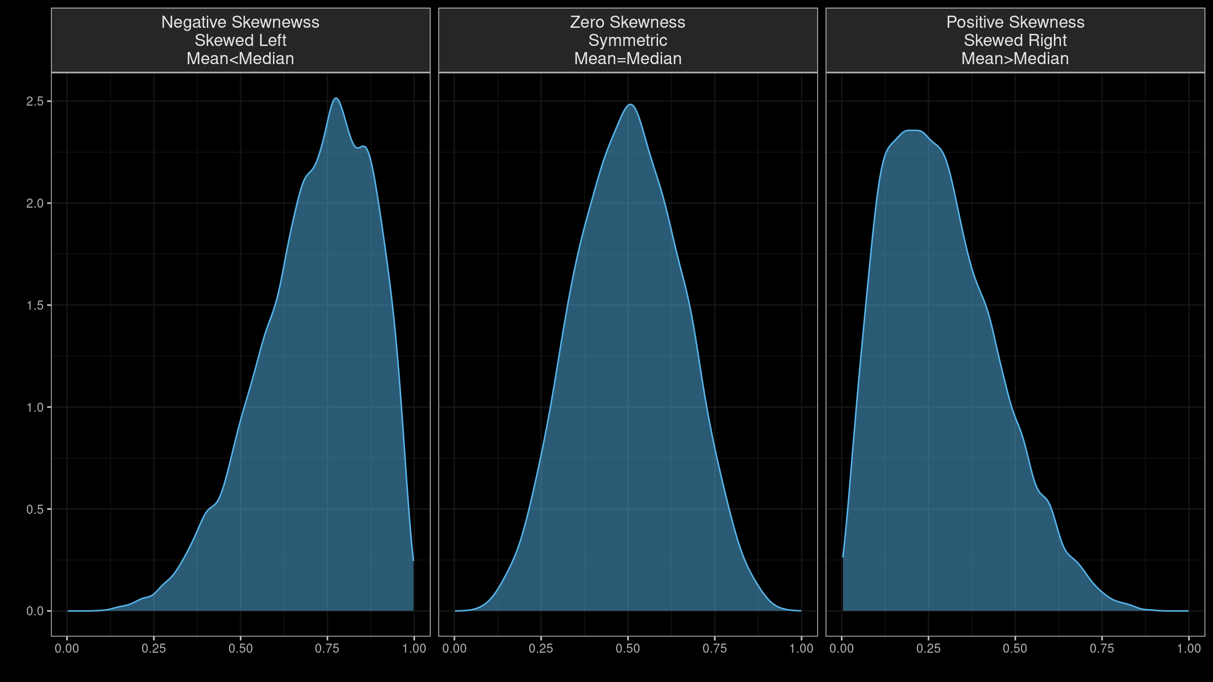
It looks extremely simple: using the skewness sign, we get an idea of the distribution form and the arrangement of the mean and the median. Unfortunately, it doesn’t always work as expected. Skewness estimation could be a highly misleading metric (even more misleading than the standard deviation). In this post, I discuss four sources of its misleadingness:

• “Skewness” is a generic term; it has multiple definitions. When a skewness value is presented, you can’t always guess the underlying equation without additional details.
• Skewness is “designed” for unimodal distributions; it’s meaningless in the case of multimodality.
• Most default skewness definitions are not robust: a single outlier could completely distort the skewness value.
• We can’t make conclusions about the locations of the mean and the median based on the skewness sign.

Greenwald-Khanna quantile estimator

The Greenwald-Khanna quantile estimator is a classic sequential quantile estimator which has the following features:

• It allows estimating quantiles with respect to the given precision $\epsilon$.
• It requires $O(\frac{1}{\epsilon} log(\epsilon N))$ memory in the worst case.
• It doesn’t require knowledge of the total number of elements in the sequence and the positions of the requested quantiles.

In this post, I briefly explain the basic idea of the underlying data structure, and share a copy-pastable C# implementation. At the end of the post, I discuss some important implementation decisions that are unclear from the original paper, but heavily affect the estimator accuracy.

P² quantile estimator rounding issue

Update: the estimator accuracy could be improved using a bunch of patches.

The P² quantile estimator is a sequential estimator that uses $O(1)$ memory. Thus, for the given sequence of numbers, it allows estimating quantiles without storing values. I already wrote a blog post about this approach and added its implementation in perfolizer. Recently, I got a bug report that revealed a flaw of the original paper. In this post, I’m going to briefly discuss this issue and the corresponding fix.