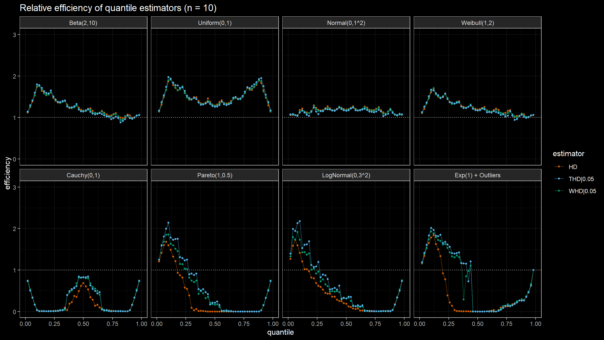
Efficiency of the winsorized and trimmed Harrell-Davis quantile estimators

In previous posts, I suggested two modifications of the Harrell-Davis quantile estimator: winsorized and trimmed. Both modifications have a higher level of robustness in comparison to the original estimator. Also, I discussed the efficiency of the Harrell-Davis quantile estimator. In this post, I’m going to continue numerical simulation and estimate the efficiency of the winsorized and trimmed modifications.

Trimmed modification of the Harrell-Davis quantile estimator

In one of the previous posts, I discussed winsorized Harrell-Davis quantile estimator. This estimator is more robust than the classic Harrell-Davis quantile estimator. In this post, I want to suggest another modification that may be better for some corner cases: the trimmed Harrell-Davis quantile estimator.

Efficiency of the Harrell-Davis quantile estimator

One of the most essential properties of a quantile estimator is its efficiency. In simple words, the efficiency describes the estimator accuracy. The Harrell-Davis quantile estimator is a good option to achieve higher efficiency. However, this estimator may provide lower efficiency in some special cases. In this post, we will conduct a set of simulations that show the actual efficiency numbers. We compare different distributions (symmetric and right-skewed, heavy-tailed and light-tailed), quantiles, and sample sizes.

Navruz-Özdemir quantile estimator

The Navruz-Özdemir quantile estimator suggests the following equation to estimate the $p^\textrm{th}$ quantile of sample $X$:

where $B_i = B(i; n, p)$ is probability mass function of the binomial distribution $B(n, p)$, $X_{(i)}$ are order statistics of sample $X$.

In this post, I derive these equations following the paper “A new quantile estimator with weights based on a subsampling approach” (2020) by Gözde Navruz and A. Fırat Özdemir. Also, I add some additional explanations, simplify the final equation, and provide reference implementations in C# and R.

Sfakianakis-Verginis quantile estimator

There are dozens of different ways to estimate quantiles. One of these ways is to use the Sfakianakis-Verginis quantile estimator. To be more specific, it’s a family of three estimators. If we want to estimate the $p^\textrm{th}$ quantile of sample $X$, we can use one of the following equations:

where $B_i = B(i; n, p)$ is probability mass function of the binomial distribution $B(n, p)$, $X_{(i)}$ are order statistics of sample $X$.

In this post, I derive these equations following the paper “A new family of nonparametric quantile estimators” (2008) by Michael E. Sfakianakis and Dimitris G. Verginis. Also, I add some additional explanations, reconstruct missing steps, simplify the final equations, and provide reference implementations in C# and R.

Winsorized modification of the Harrell-Davis quantile estimator

The Harrell-Davis quantile estimator is one of my favorite quantile estimators because of its efficiency. It has a small mean square error which allows getting accurate estimations. However, it has a severe drawback: it’s not robust. Indeed, since the estimator includes all sample elements with positive weights, its breakdown point is zero.

In this post, I want to suggest modifications of the Harrell-Davis quantile estimator which increases its robustness keeping almost the same level of efficiency.

Misleading standard deviation

The standard deviation may be an extremely misleading metric. Even minor deviations from normality could make it completely unreliable and deceiving. Let me demonstrate this problem using an example.

Below you can see three density plots of some distributions. Could you guess their standard deviations?

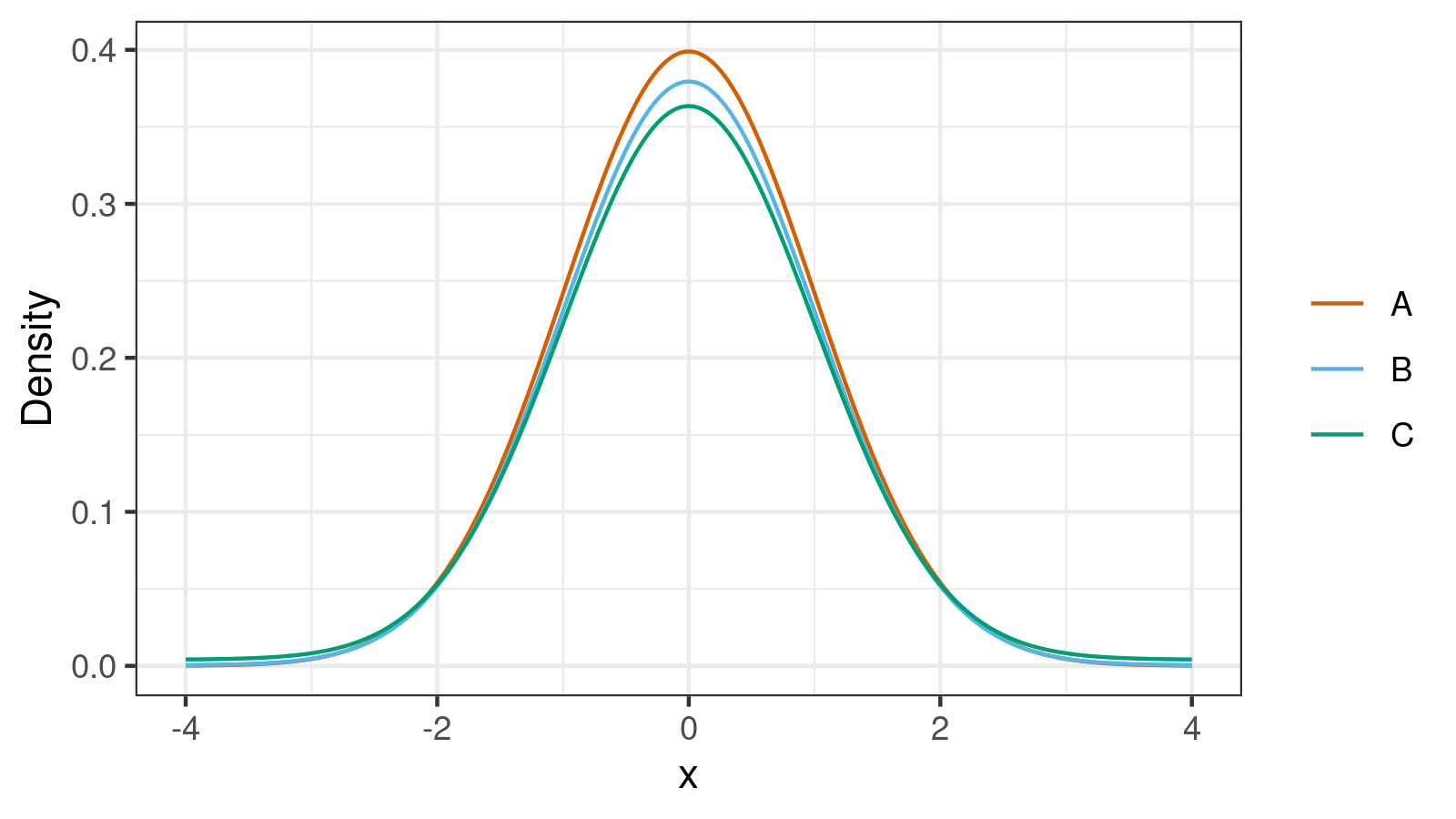
The correct answers are $1.0, 3.0, 11.0$. And here is a more challenging problem: could you match these values with the corresponding distributions?

Unbiased median absolute deviation based on the Harrell-Davis quantile estimator

The median absolute deviation ($\textrm{MAD}$) is a robust measure of scale. In the previous post, I showed how to use the unbiased version of the $\textrm{MAD}$ estimator as a robust alternative to the standard deviation. “Unbiasedness” means that such estimator’s expected value equals the true value of the standard deviation. Unfortunately, there is such thing as the bias–variance tradeoff: when we remove the bias of the $\textrm{MAD}$ estimator, we increase its variance and mean squared error ($\textrm{MSE}$).

In this post, I want to suggest a more efficient unbiased $\textrm{MAD}$ estimator. It’s also a consistent estimator for the standard deviation, but it has smaller $\textrm{MSE}$. To build this estimator, we should replace the classic “straightforward” median estimator with the Harrell-Davis quantile estimator and adjust bias-correction factors. Let’s discuss this approach in detail.

Unbiased median absolute deviation

The median absolute deviation ($\textrm{MAD}$) is a robust measure of scale. For distribution $X$, it can be calculated as follows:

where $C$ is a constant scale factor. This metric can be used as a robust alternative to the standard deviation. If we want to use the $\textrm{MAD}$ as a consistent estimator for the standard deviation under the normal distribution, we should set

where $\Phi^{-1}$ is the quantile function of the standard normal distribution (or the inverse of the cumulative distribution function). If $X$ is the normal distribution, we get $\textrm{MAD} = \sigma$ where $\sigma$ is the standard deviation.

Now let’s consider a sample $x = \{ x_1, x_2, \ldots x_n \}$. Let’s denote the median absolute deviation for a sample of size $n$ as $\textrm{MAD}_n$. The corresponding equation looks similar to the definition of $\textrm{MAD}$ for a distribution:

Let’s assume that $\textrm{median}$ is the straightforward definition of the median (if $n$ is odd, the median is the middle element of the sorted sample, if $n$ is even, the median is the arithmetic average of the two middle elements of the sorted sample). We still can use $C_n = C_{\infty}$ for extremely large sample sizes. However, for small $n$, $\textrm{MAD}_n$ becomes a biased estimator. If we want to get an unbiased version, we should adjust the value of $C_n$.

In this post, we look at the possible approaches and learn the way to get the exact value of $C_n$ that makes $\textrm{MAD}_n$ unbiased estimator of the median absolute deviation for any $n$.

Comparing distribution quantiles using gamma effect size

There are several ways to describe the difference between two distributions. Here are a few examples:

• Effect sizes based on differences between means (e.g., Cohen’s d, Glass’ Δ, Hedges’ g)
• The shift and ration functions that estimate differences between matched quantiles.

In one of the previous post, I described the gamma effect size which is defined not for the mean but for quantiles. In this post, I want to share a few case studies that demonstrate how the suggested metric combines the advantages of the above approaches.