Weighted Hodges-Lehmann location estimator and mixture distributions

The classic non-weighted Hodges-Lehmann location estimator of a sample $\mathbf{x} = (x_1, x_2, \ldots, x_n)$ is defined as follows:

where $\operatorname{median}$ is the sample median. Previously, we have defined a weighted version of the Hodges-Lehmann location estimator as follows:

where $\mathbf{w} = (w_1, w_2, \ldots, w_n)$ is the vector of weights, $\operatorname{wmedian}$ is the weighted median. For simplicity, in the scope of the current post, Hyndman-Fan Type 7 quantile estimator is used as the base for the weighted median.

In this post, we consider a numerical simulation in which we compare sampling distribution of $\operatorname{HL}$ and $\operatorname{WHL}$ in a case of mixture distribution.

Carling’s Modification of the Tukey's fences

Let us consider the classic problem of outlier detection in one-dimensional sample. One of the most popular approaches is Tukey’s fences, that defines the following range:

where $Q_1$ and $Q_3$ are the first and the third quartiles of the given sample.

All the values outside the given range are classified as outliers. The typical values of $k$ are $1.5$ for “usual outliers” and $3.0$ for “far out” outliers. In the classic Tukey’s fences approach, $k$ is often a predefined constant. However, there are alternative approaches that define $k$ dynamically based on the given sample. One of the possible variations of Tukey’s fences is Carling’s modification that defines $k$ as follows:

where $n$ is the sample size.

In this post, we compare the classic Tukey’s fences with $k=1.5$ and $k=3.0$ against Carling’s modification.

Central limit theorem and log-normal distribution

It is inconvenient to work with samples from a distribution of unknown form. Therefore, researchers often switch to considering the sample mean value and hope that thanks to the central limit theorem, the distribution of the sample means should be approximately normal. They say that if we consider samples of size $n \geq 30$, we can expect practically acceptable convergence to normality thanks to Berry–Esseen theorem. Indeed, this statement is almost valid for many real data sets. However, we can actually expect the applicability of this approach only for light-tailed distributions. In the case of heavy-tailed distributions, converging to normality is so slow, that we cannot imply the normality assumption for the distribution of the sample means. In this post, I provide an illustration of this effect using the log-normal distribution.

Hodges-Lehmann Gaussian efficiency: location shift vs. shift of locations

Let us consider two samples $\mathbf{x} = (x_1, x_2, \ldots, x_n)$ and $\mathbf{y} = (y_1, y_2, \ldots, y_m)$. The one-sample Hodges-Lehman location estimator is defined as the median of the Walsh (pairwise) averages:

For these two samples, we can also define the shift between these two estimations:

The two-sample Hodges-Lehmann location shift estimator is defined as the median of pairwise differences:

Previously, I already compared the location shift estimator with the difference of median estimators (1, 2). In this post, I compare the difference between two location estimations and the shift estimations in terms of Gaussian efficiency. Before I started this study, I expected that $\operatorname{HL}$ should be more efficient than $\Delta_{\operatorname{HL}}$. Let us find out if my intuition is correct or not!

Thoughts on automatic statistical methods and broken assumptions

Ratio estimator based on the Hodges-Lehmann approach

For two samples $\mathbf{x} = ( x_1, x_2, \ldots, x_n )$ and $\mathbf{y} = ( y_1, y_2, \ldots, y_m )$, the Hodges-Lehmann location shift estimator is defined as follows:

Now, let us consider the problem of estimating the ratio of the location measures instead of the shift between them. While there are multiple approaches to providing such an estimation, one of the options that can be considered is based on the Hodges-Lehmann ideas.

Weighted Mann-Whitney U test, Part 2

Previously, I suggested a weighted version of the Mann–Whitney $U$ test. The distribution of the weighted normalized $U_\circ^\star$ can be obtained via bootstrap. However, it is always nice if we can come up with an exact solution for the statistic distribution or at least provide reasonable approximations. In this post, we start exploring this distribution.

Exploring the power curve of the Cucconi test

The Cucconi test is a nonparametric two-sample test that compares both location and scale. It is a classic example of the family of tests that perform such a comparison simultaneously instead of combining the results of a location test and a scale test. Intuitively, such an approach should fit well unimodal distributions. Moreover, it has the potential to outperform more generic nonparametric tests that do not rely on the unimodality assumption.

In this post, we briefly show the equations behind the Cucconi test and present a power curve that compares it with the Student’s t-test and the Mann-Whitney U test under normality.

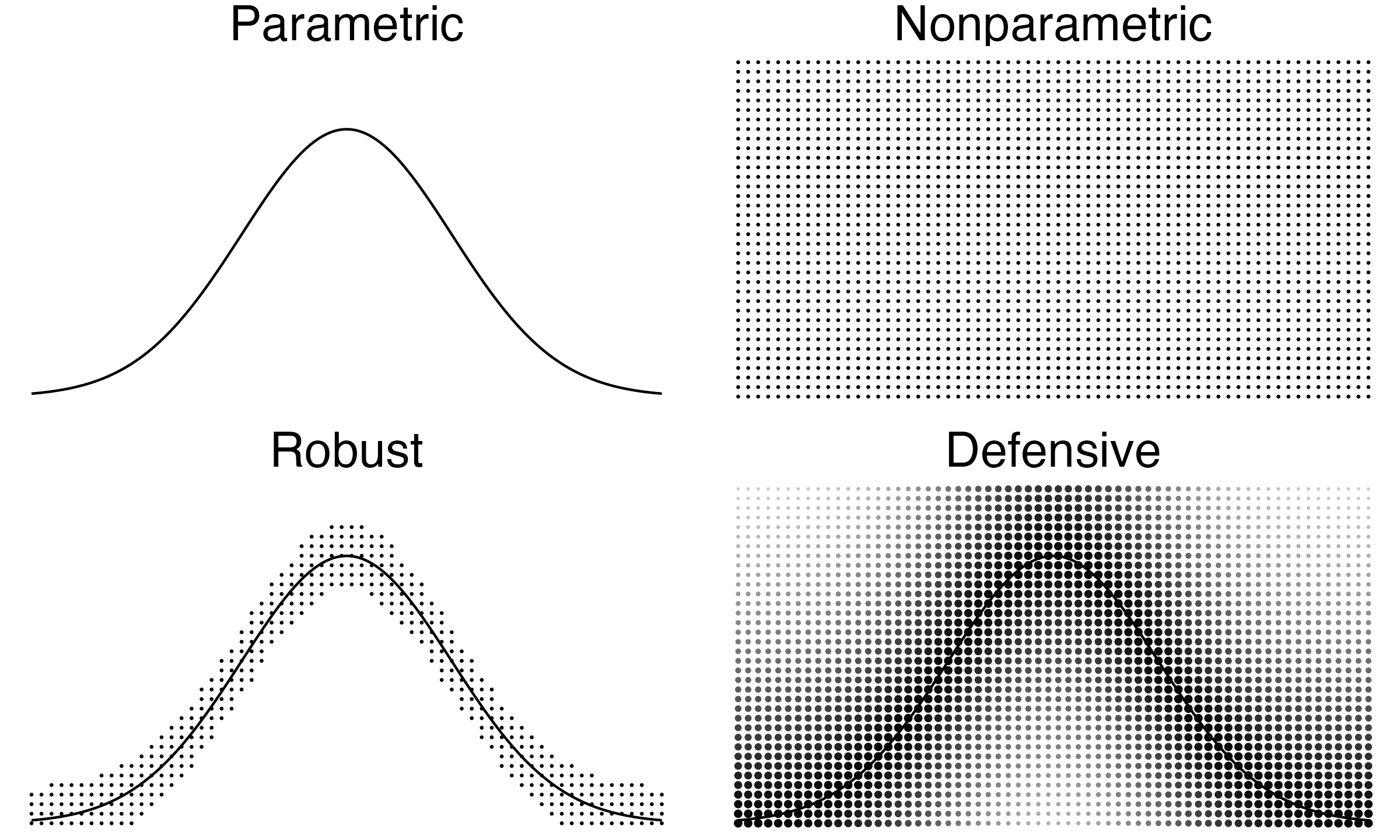
Parametric, Nonparametric, Robust, and Defensive statistics

Recently, I started writing about defensive statistics. The methodology allows having parametric assumptions, but it adjusts statistical methods so that they continue working even in the case of huge deviations from the declared assumptions. This idea sounds quite similar to nonparametric and robust statistics. In this post, I briefly explain the difference between different statistical methodologies.