Effect Sizes and Asymmetry
Cohen’s d is one of the most popular measures of the effect size. Unfortunately, it was designed for the normal distribution, which may make it a misleading measure in the non-normal case. And the real distributions are Normalitynever normal. When we discuss deviations from normality, we should treat the illusion of normality not as an atomic mental construction, but rather as a set of independent assumptions, each of which may be violated independently. In this post, I take a look at what kind of issues we may have when the symmetry assumption is heavily violated.
First of all, let us choose the measure of the effect size. While Cohen’s d provides a well-adopted scale of values, it’s not robust. First of all, we solve the robustness issue. When we work with the “difference family” of effect sizes, we essentially divide the measure of shift in locations by the measure of spread. Cohen’s d is based on the difference in arithmetic means and the pooled standard deviation. We can customize it by adopting the Hodges-Lehmann EstimatorHodges-Lehmann Estimator as the measure of shift and the Shamos EstimatorShamos Estimator as the measure of spread. It helps resolve the robustness problem.
Now let us discuss the asymmetry problem. For the model distribution, we consider the exponential one. Let $\mathbf{x}_A$ be a sample from the scaled and shifted exponential distribution:
$$ \mathbf{x}_A \in \left( 3 \cdot \operatorname{Exp}(1) - 3.544861 \right). $$Next, we define three additional samples as follows:
$$ \mathbf{y}_A = -\mathbf{x}_A,\quad \mathbf{x}_B = -\mathbf{x}_A - 2,\quad \mathbf{y}_B = -\mathbf{x}_B. $$Therefore, we have the following Hodges-Lehmann estimations:
$$ \operatorname{HL}(\mathbf{x}_A) = \operatorname{HL}(\mathbf{x}_B) = -1,\quad \operatorname{HL}(\mathbf{y}_A) = \operatorname{HL}(\mathbf{y}_B) = 1. $$The estimated density plots of these samples are shown below (vertical lines correspond to the Hodges–Lehmann estimations):
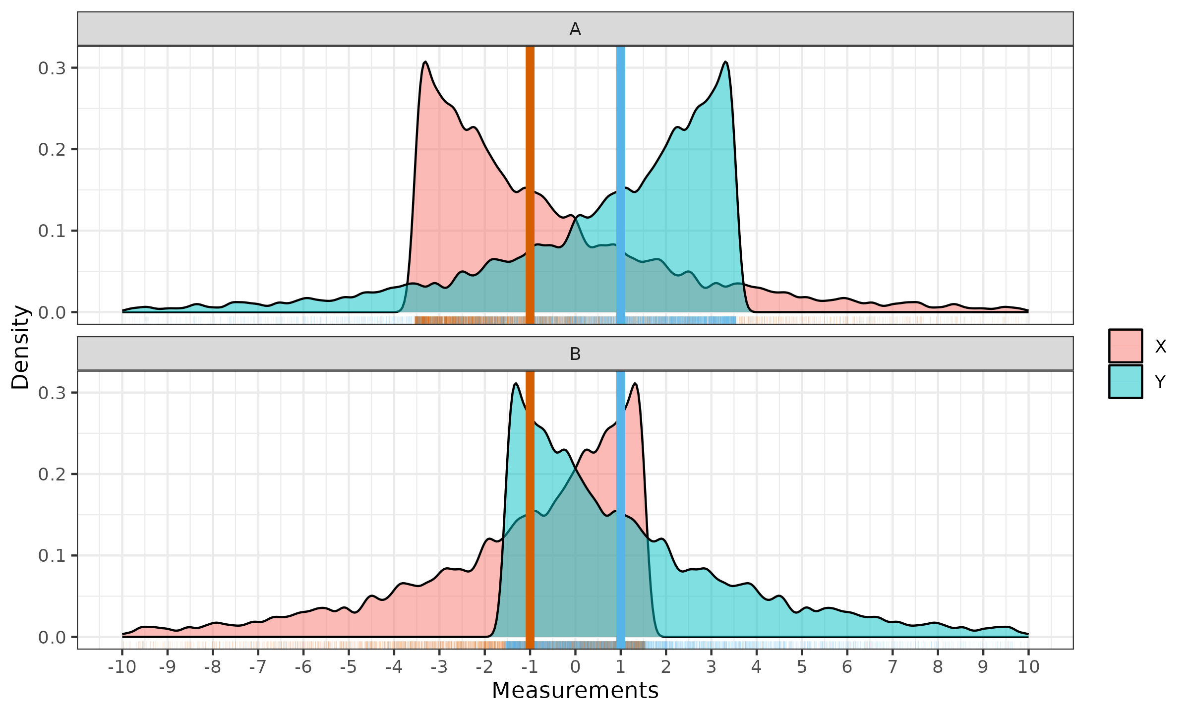
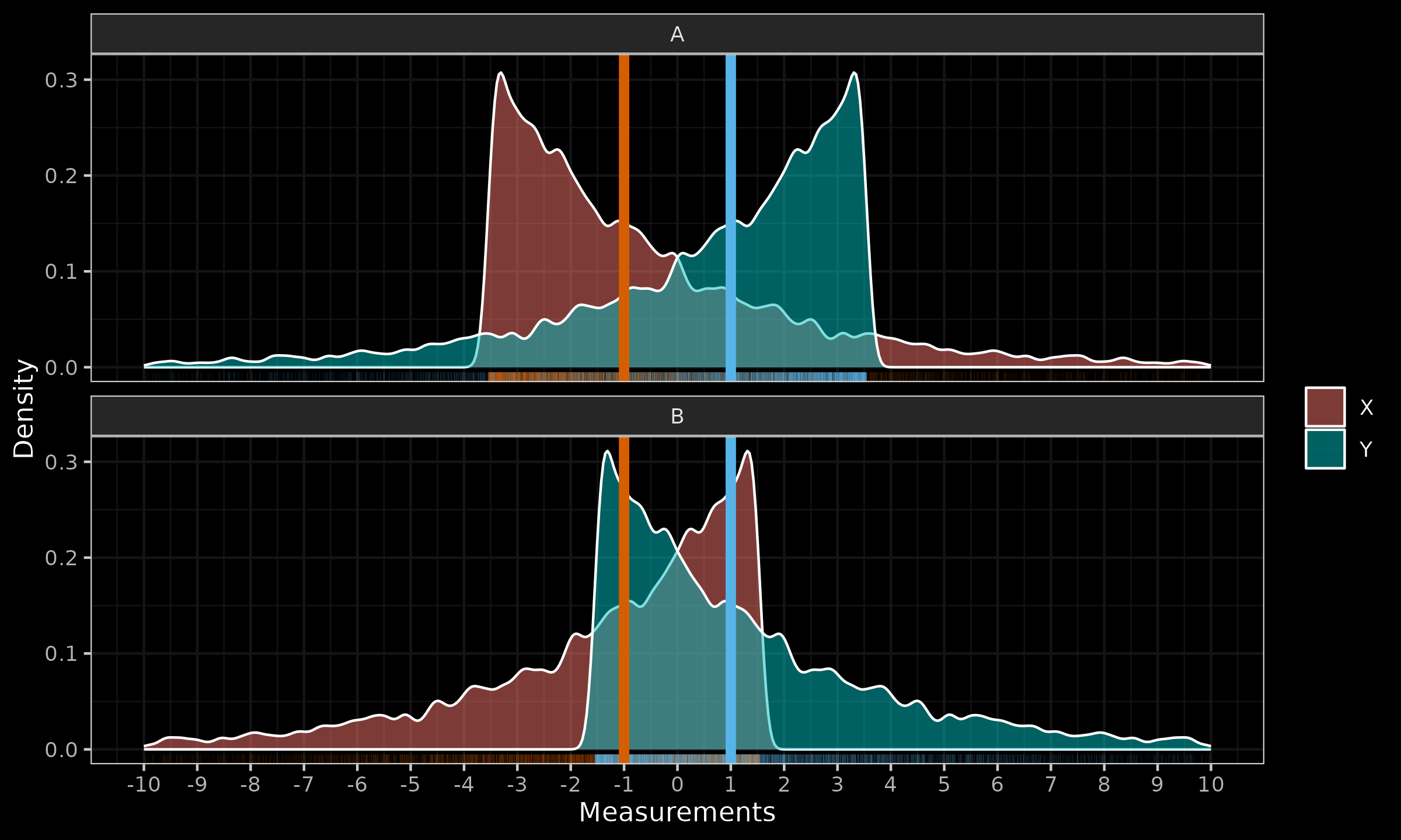
While $\left(\mathbf{x}_A\; \textrm{vs.}\; \mathbf{y}_A\right)$ and $\left(\mathbf{x}_B\; \textrm{vs.}\; \mathbf{y}_B\right)$ feel like quite different distributions, they are not so different in terms of the effect size. Indeed, all four samples have the same shape, the only difference is about shifts and reflections. Thus, the spread of all samples is the same regardless of the scale estimator. The Hodges-Lehmann shift is identical for both pairs:
$$ \operatorname{HL}(\mathbf{x}_A, \mathbf{y}_A) = \operatorname{HL}(\mathbf{x}_B, \mathbf{y}_B) \approx 2. $$Therefore, we use the previously introduced robust measure of effect size, and we will also have identical results:
$$ \operatorname{ES}(\mathbf{x}_A, \mathbf{y}_A) = \operatorname{ES}(\mathbf{x}_B, \mathbf{y}_B). $$If we rely on the effect size as the only measure of the difference, we will not be able to distinguish the presented cases. Such an approach may work fine with slight deviations from normality, which means slight deviations from the symmetric model. However, once strong asymmetry is introduced, a single effect size estimation is not capable of reliably describing the investigated difference.