Beta distribution highest density interval of the given width
In one of the previous posts, I discussed the idea of the trimmed Harrell-Davis quantile estimator based on the highest density interval of the given width. Since the Harrell-Davis quantile estimator uses the Beta distribution, we should be able to find the beta distribution highest density interval of the given width. In this post, I will show how to do this.
The problem
The Beta distribution is defined by two parameters $\alpha$ and $\beta$. We want to find its highest density interval of size $w \in [0; 1]$. To be more formal, we want to build a function $\operatorname{HDI}(\alpha, \beta, w)$ that returns a highest density interval $[L;R]$ such as $R-L=w$:
$$ \operatorname{HDI}(\alpha, \beta, w) = [L; R] $$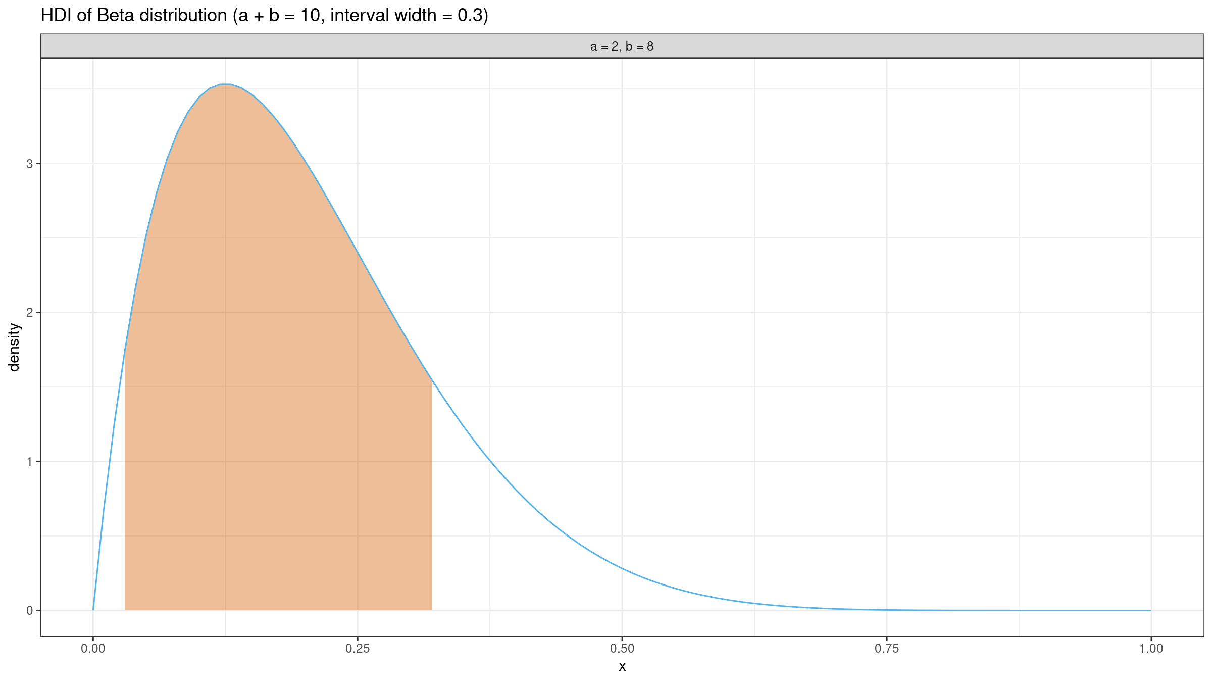
Getting the mode location
First of all, let’s recall the equations for the mode of the beta distribution:
$$ M = \operatorname{Mode}_{\alpha, \beta} = \begin{cases} \frac{\alpha - 1}{\alpha + \beta - 2} & \textrm{for }\, \alpha > 1,\, \beta > 1,\\ 0 & \textrm{for }\, \alpha \leq 1,\, \beta > 1,\\ 1 & \textrm{for }\, \alpha > 1,\, \beta \leq 1,\\ \{0, 1 \} & \textrm{for }\, \alpha < 1,\, \beta < 1,\\ \textrm{any value in } (0, 1) & \textrm{for }\, \alpha = 1,\, \beta = 1. \end{cases} $$The actual value of $\operatorname{HDI}(\alpha, \beta, w)$ depends on the specific case from the above list which defines the mode location. Let’s discuss each of these cases.
Degenerate case
The degenerate case is described by the following condition:
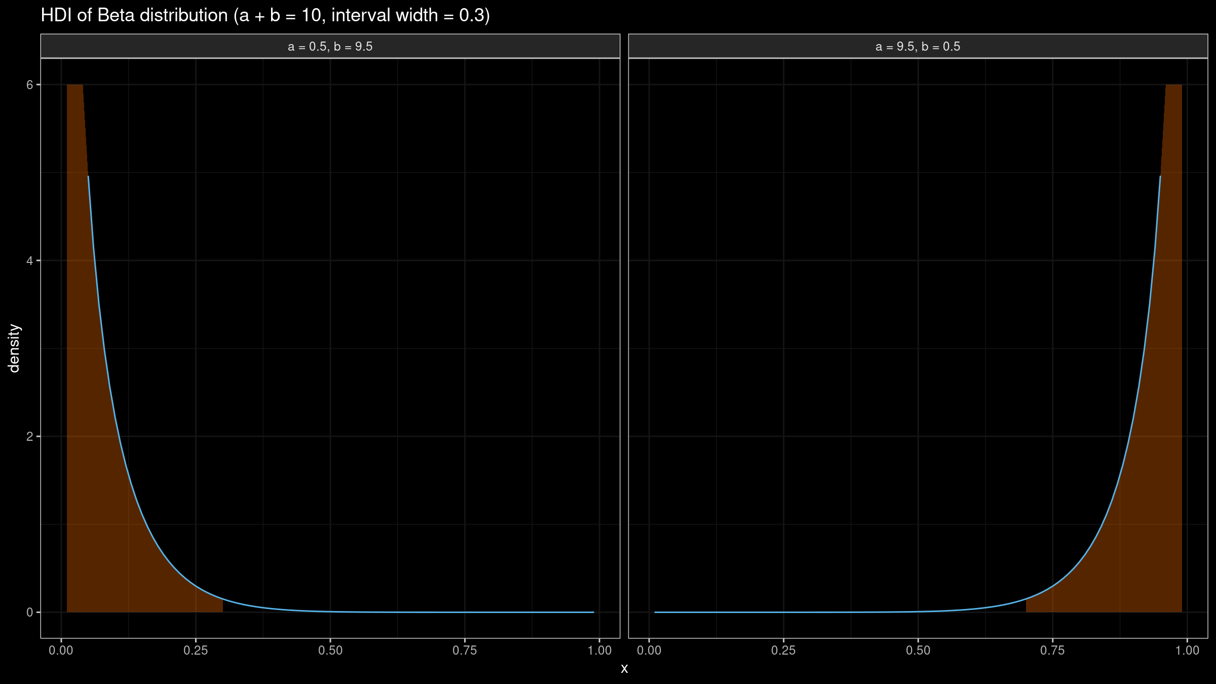
$$ \alpha \leq 1, \quad \beta \leq 1. $$When $\alpha < 1,\, \beta < 1$, the beta distribution has two modes: $0$ and $1$. Thus, there are two highest density intervals: $[0; w]$ and $[1 - w; 1]$.
When $\alpha = 1,\, \beta = 1$, all the values in $[0;1]$ could be considered as modes because the density function has a constant value. Thus, all the intervals of the same width cover the same density area.
Border case
The border case is described by the following condition:
$$ \alpha \leq 1, \, \beta > 1 \quad \lor \quad \alpha > 1, \, \beta \leq 1. $$This condition covers two cases in which the highest density interval “is attached” to one of the borders:
- $\alpha \leq 1, \, \beta > 1: \quad M = 0, \quad \operatorname{HDI}(\alpha, \beta, w) = [0; w]$
- $\alpha > 1, \, \beta \leq 1: \quad M = 1, \quad \operatorname{HDI}(\alpha, \beta, w) = [1 - w; 1]$

Middle case
The “middle” case is described by the following condition:
$$ \alpha > 1, \quad \beta > 1. $$In this case, the highest density interval is somewhere in the middle of $[0;1]$:

Since the density function of the beta distribution is a unimodal function, it consists of two segments:
- $[0, M]$: Monotonically increased segment
- $[M, 1]$: Monotonically decreased segment
Since $R - L = w$, we could also conclude that
$$ L \in [M - w; 1 - w], \quad R \in [w; M + w]. $$Thus,
$$ L \in [\max(0, M - w);\; \min(M, 1 - w)], \quad R \in [\max(w, M);\; \min(1, M + w)]. $$The density function of the Beta distribution is also known:
$$ f(x) = \dfrac{x^{\alpha - 1} (1 - x)^{\beta - 1}}{\textrm{B}(\alpha, \beta)}, \quad \textrm{B}(\alpha, \beta) = \dfrac{\Gamma(\alpha)\Gamma(\beta)}{\Gamma(\alpha + \beta)}. $$It’s easy to see that for the highest density interval $[L; R]$ the following condition is true:
$$ f(L) = f(R) $$The left border $L$ of this interval could be found as a solution of the following equation:
$$ f(x) = f(x + w), \quad \textrm{where }\, x \in [\max(0, M - w);\; \min(M, 1 - w)]. $$The left side of the equation is monotonically increasing, the right side is monotonically decreasing. The equation has exactly one solution which could be easily found numerically using the binary search algorithm.
Numerical simulations
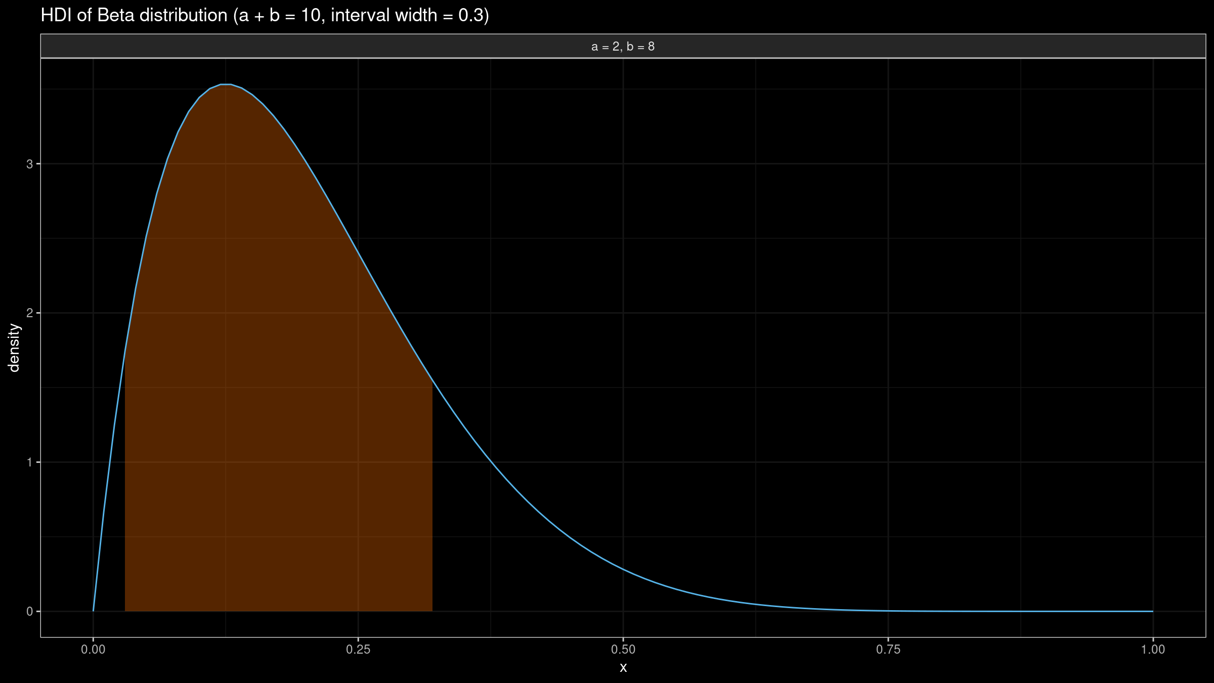
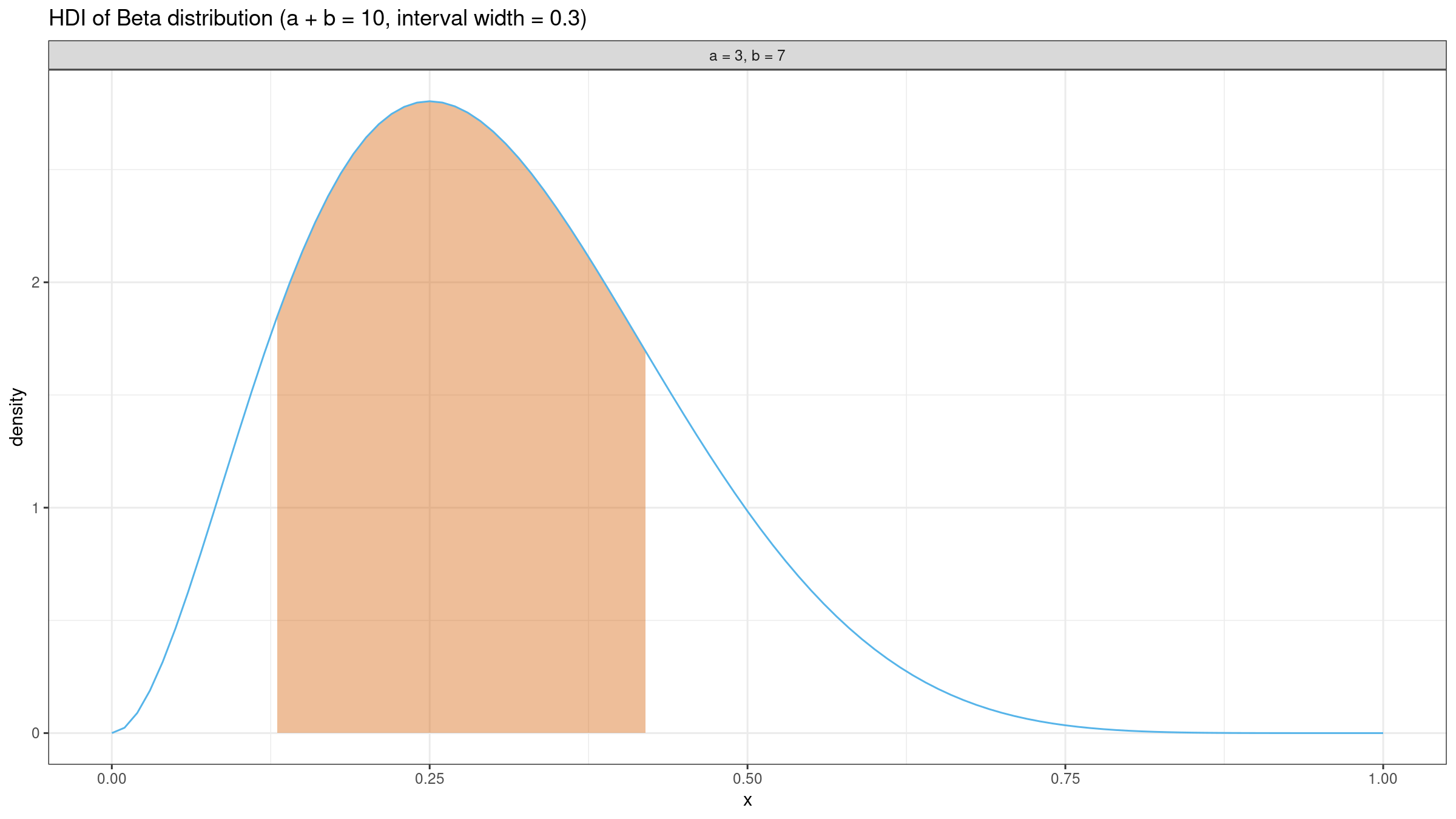
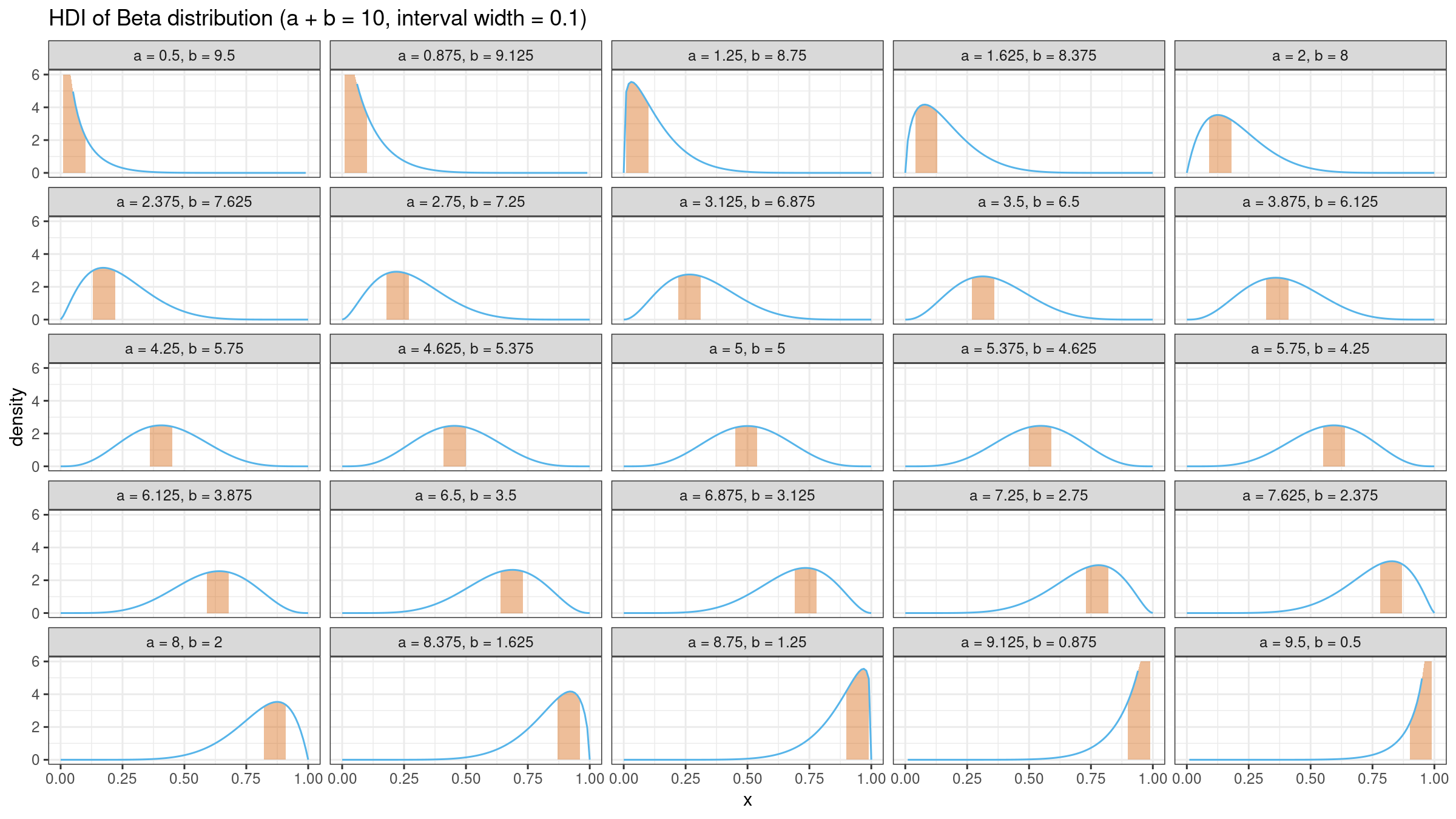
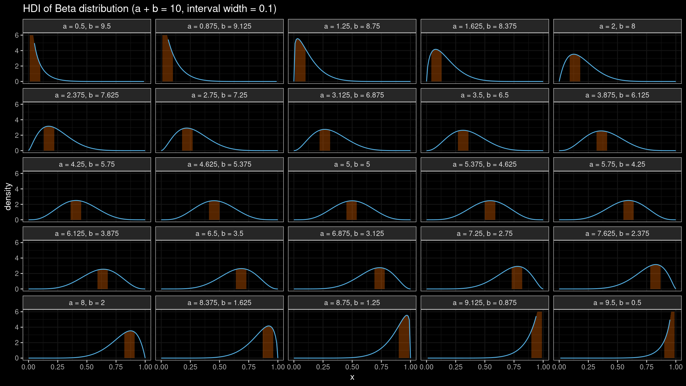
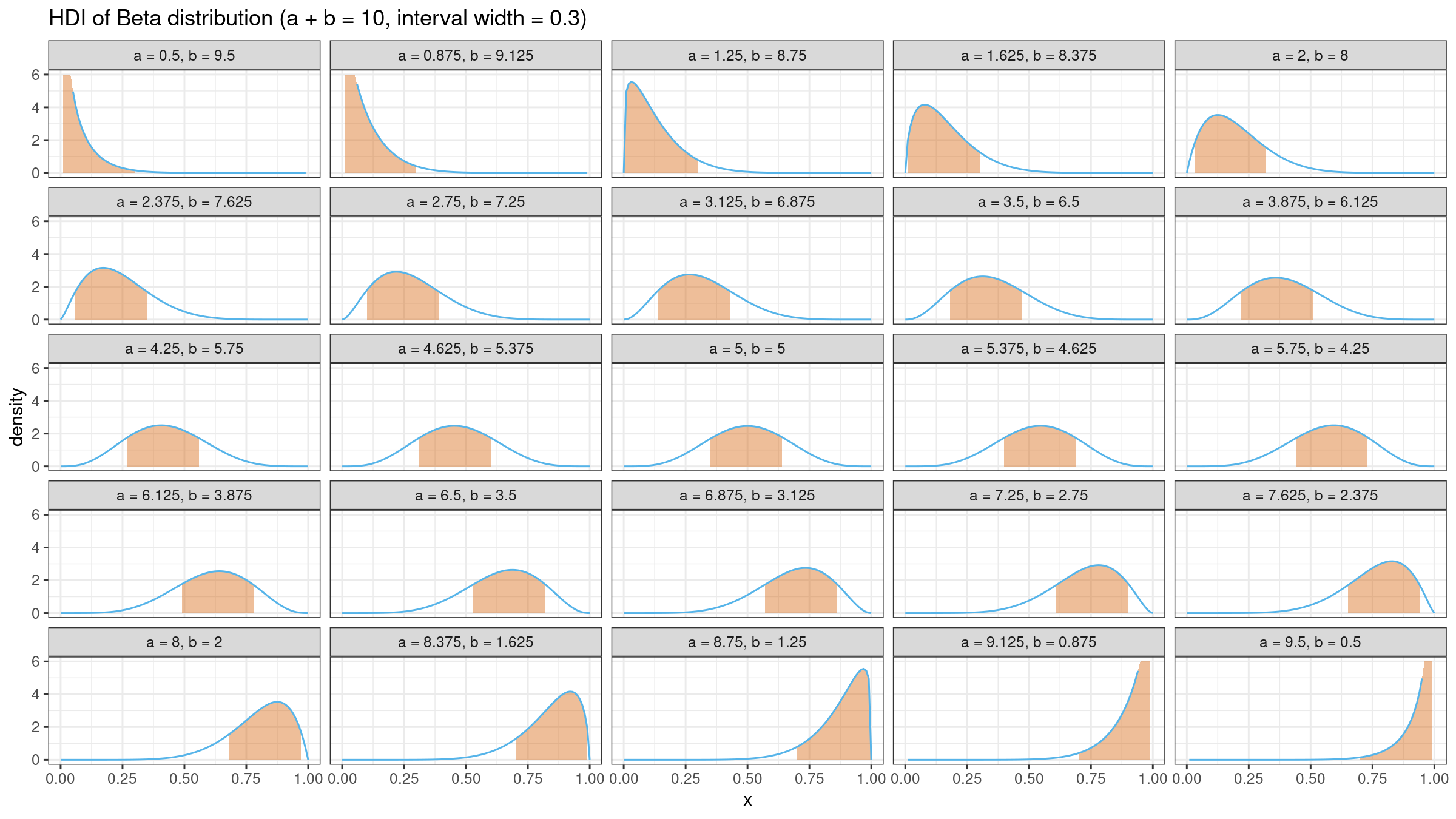
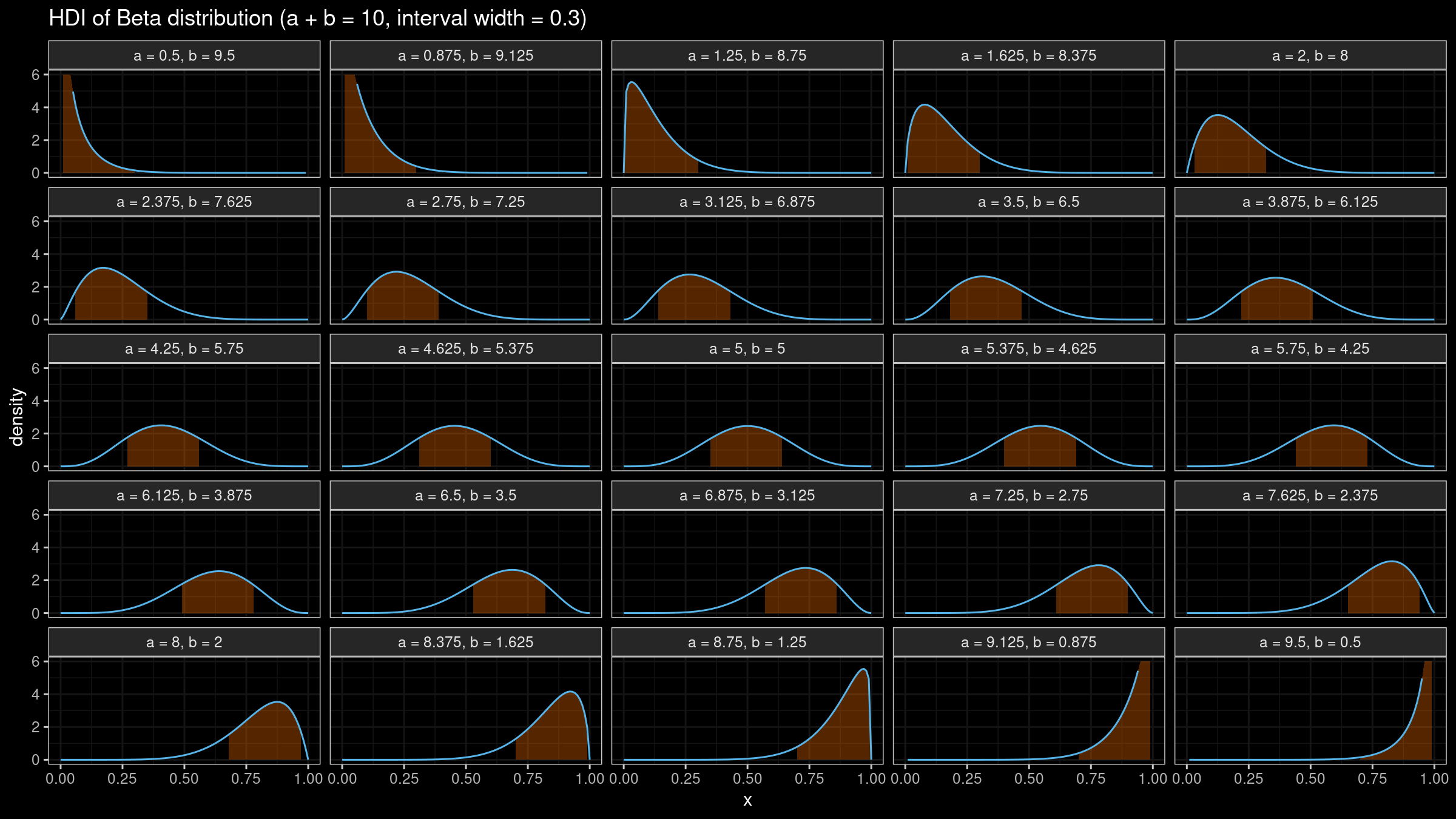
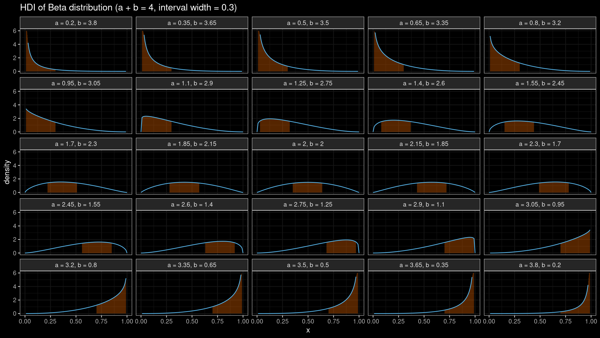
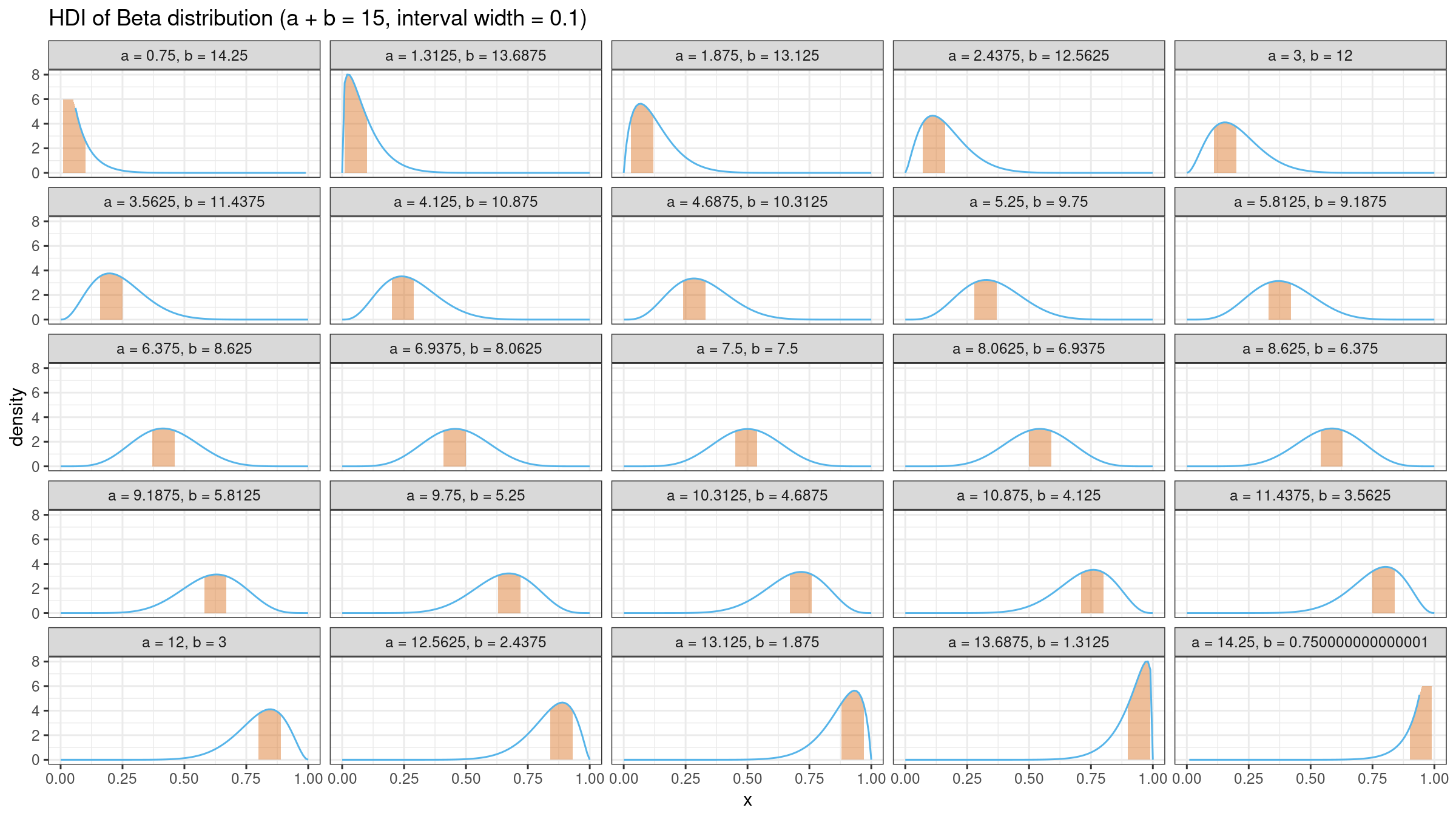
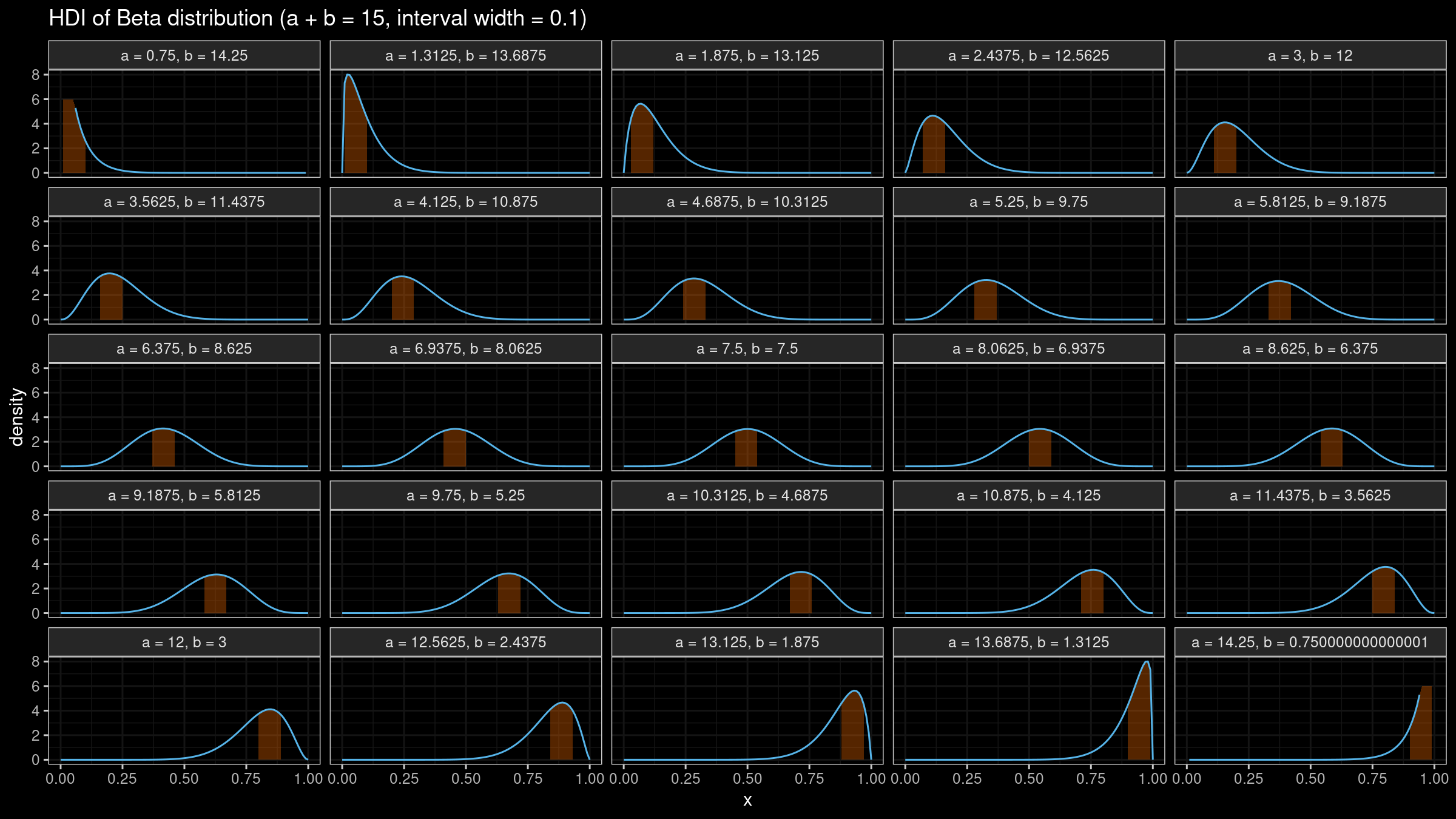
Below you can see beta function highest density intervals for different parameter configurations:

Reference implementation
Here is a reference R implementation of the above algorithm:
getBetaHdi <- function(a, b, width) {
  eps <- 1e-9
  if (a < 1 + eps & b < 1 + eps) # Degenerate case
    return(c(NA, NA))
  if (a < 1 + eps & b > 1) # Left border case
    return(c(0, width))
  if (a > 1 & b < 1 + eps) # Right border case
    return(c(1 - width, 1))

  # Middle case
  mode <- (a - 1) / (a + b - 2)
  pdf <- function(x) dbeta(x, a, b)

  l <- uniroot(
    f = function(x) pdf(x) - pdf(x + width),
    lower = max(0, mode - width),
    upper = min(mode, 1 - width)
    )$root
  r <- l + width
  return(c(l, r))
}