Carling’s Modification of the Tukey's fences
Let us consider the classic problem of outlier detection in one-dimensional sample. One of the most popular approaches is Tukey’s fences, that defines the following range:
$$ [Q_1 - k(Q_3 - Q_1);\; Q_3 + k(Q_3 - Q_1)], $$where $Q_1$ and $Q_3$ are the first and the third quartiles of the given sample.
All the values outside the given range are classified as outliers. The typical values of $k$ are $1.5$ for “usual outliers” and $3.0$ for “far out” outliers. In the classic Tukey’s fences approach, $k$ is often a predefined constant. However, there are alternative approaches that define $k$ dynamically based on the given sample. One of the possible variations of Tukey’s fences is Carling’s modification that defines $k$ as follows:
$$ k = \frac{17.63n - 23.64}{7.74n - 3.71}, $$where $n$ is the sample size.
In this post, we compare the classic Tukey’s fences with $k=1.5$ and $k=3.0$ against Carling’s modification.
First of all, let us look at the values of $k$ in the Carling’s modification:
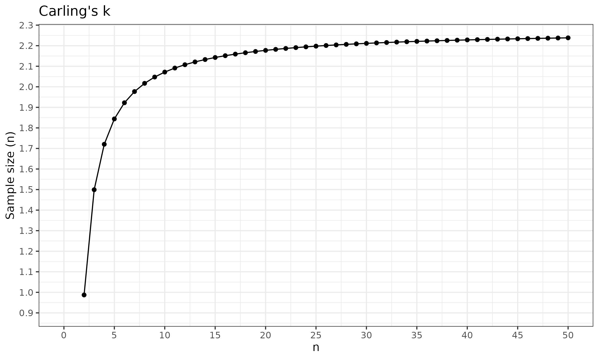
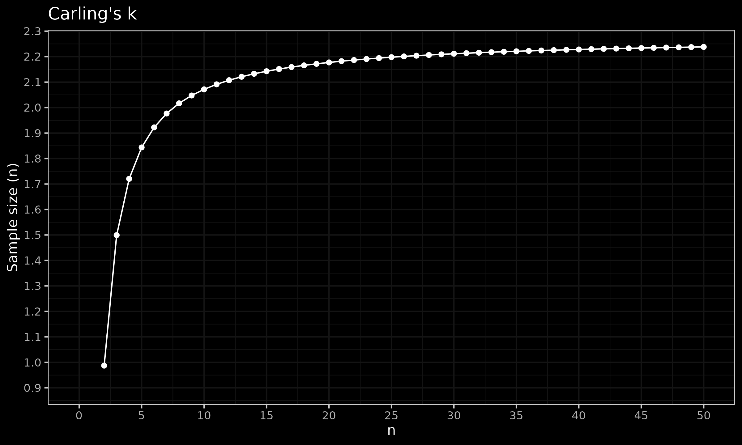
As we can see, $k$ starts at $\approx 0.99$ for $n=2$ and quickly converges to $\approx 2.28$ for large $k$.
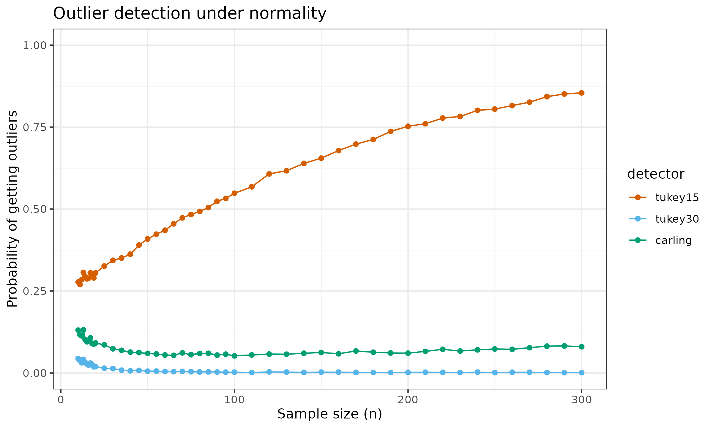
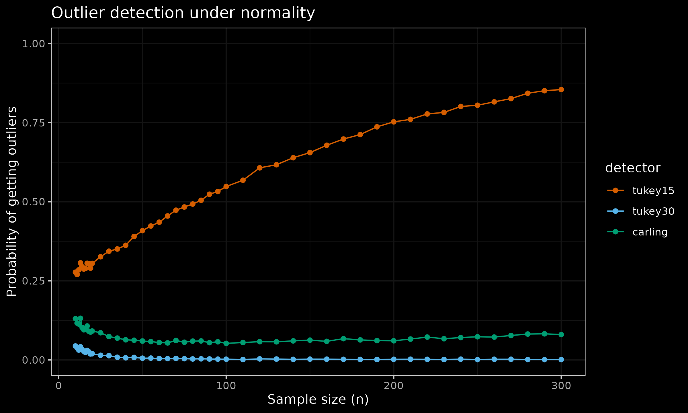
Now let us conduct the following numerical simulations:
- Enumerate various fence-based outlier detector: Tukey’s fences with $k=1.5$, $k=3.0$ and the Carling’s modification.
- Enumerate various sample sizes from $n=2$ to $n=300$.
- For each detector, generate multiple samples from the standard normal distribution, and calculate the percentage of samples that contain at least one outlier based on the given detector.
Here are the results:
Second part: Carling’s Modification of the Tukey's fences, Part 2
By Andrey Akinshin
·
2025-11-12Carling’s Modification of the Tukey's fences, Part 2.
The Carling’s modification gives a reasonable and adaptive trade-off. The ratio of samples with detected outliers quickly converges to ≈0.08 even for large values of n. If this value doesn’t satisfy our research goals, further modifications can be applied, see [Carling2000] for details.
References
- [Carling2000]
Carling, Kenneth. “Resistant outlier rules and the non-Gaussian case.” Computational Statistics & Data Analysis 33, no. 3 (2000): 249-258.
DOI: 10.1016/S0167-9473(99)00057-2