Carling’s Modification of the Tukey's fences, Part 2

In Carling’s Modification of the Tukey's fences
By Andrey Akinshin · 2023-09-26Carling’s Modification of the Tukey's fences, I evaluated the probability of outlier detection for samples from the Normal distribution across different outlier detectors. I performed numerical simulations for small sample sizes, then confidently extrapolated the results to larger samples. As it turns out, this approach led to the wrong conclusion. This post corrects that error by extending the simulation to much larger sample sizes and updating the analysis accordingly.

Introduction

Outlier detection in one-dimensional samples requires choosing appropriate thresholds for identifying unusual values. Tukey’s fences is one widely used method that defines an interval based on the interquartile range:

$$ [Q_1 - k(Q_3 - Q_1);\; Q_3 + k(Q_3 - Q_1)], $$

where $Q_1$ and $Q_3$ are the first and third quartiles of the sample. Any value falling outside this interval is classified as an outlier.

The parameter $k$ controls the sensitivity of the detector. Common choices are $k = 1.5$ for detecting typical outliers and $k = 3.0$ for identifying extreme values. In the standard formulation, $k$ remains fixed regardless of sample size. This fixed approach ignores that quartile estimates become more precise with larger samples.

Carling’s modification ( Resistant outlier rules and the non-Gaussian case
By Kenneth Carling · 2000-05-01carling2000) makes $k$ depend on the sample size $n$:

$$ k = \frac{17.63n - 23.64}{7.74n - 3.71}. $$

As $n$ increases, this expression converges to approximately $2.28$, providing a sample-size-dependent threshold. This post compares the performance of the fixed thresholds ($k = 1.5$ and $k = 3.0$) against Carling’s adaptive approach through numerical simulation.

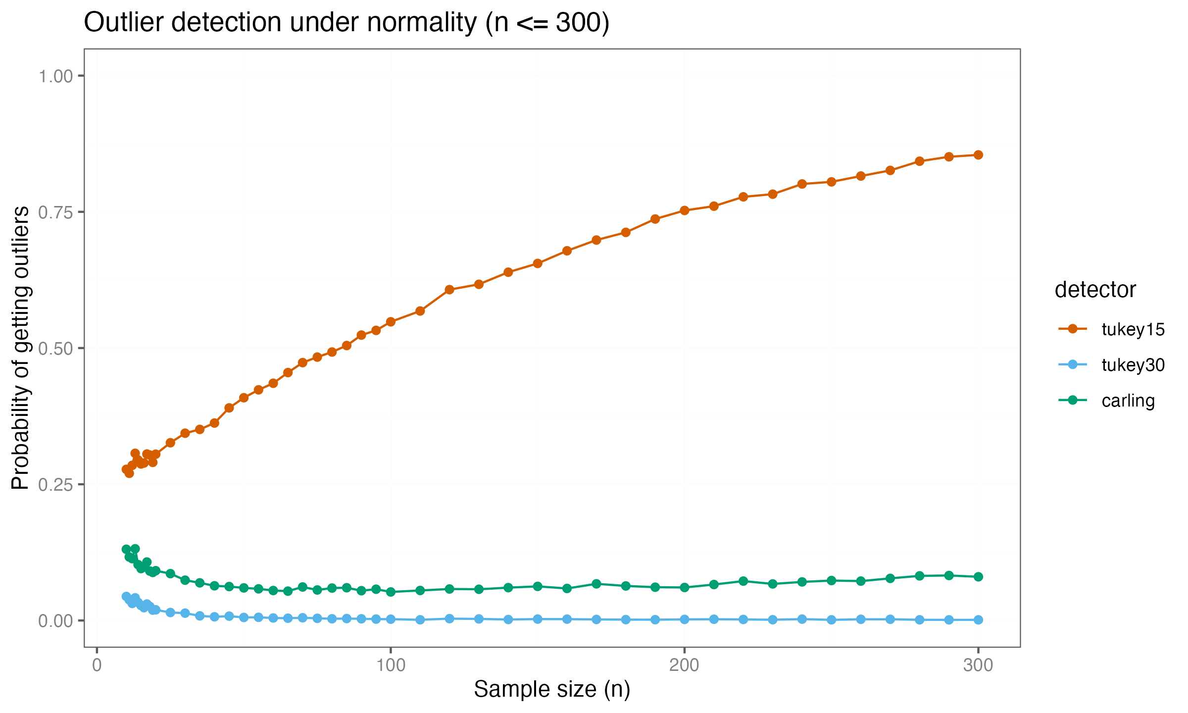
Numerical simulation

The original analysis in Carling’s Modification of the Tukey's fences
By Andrey Akinshin · 2023-09-26Carling’s Modification of the Tukey's fences examined sample sizes up to $n = 300$. At this scale, the simulation suggested that both the $k = 3.0$ threshold and Carling’s method converge toward near-zero detection rates.

Extending the simulation to larger sample sizes shows this conclusion is incorrect. Expanding the analysis to $n \leq 10\,000$ reveals a different pattern:

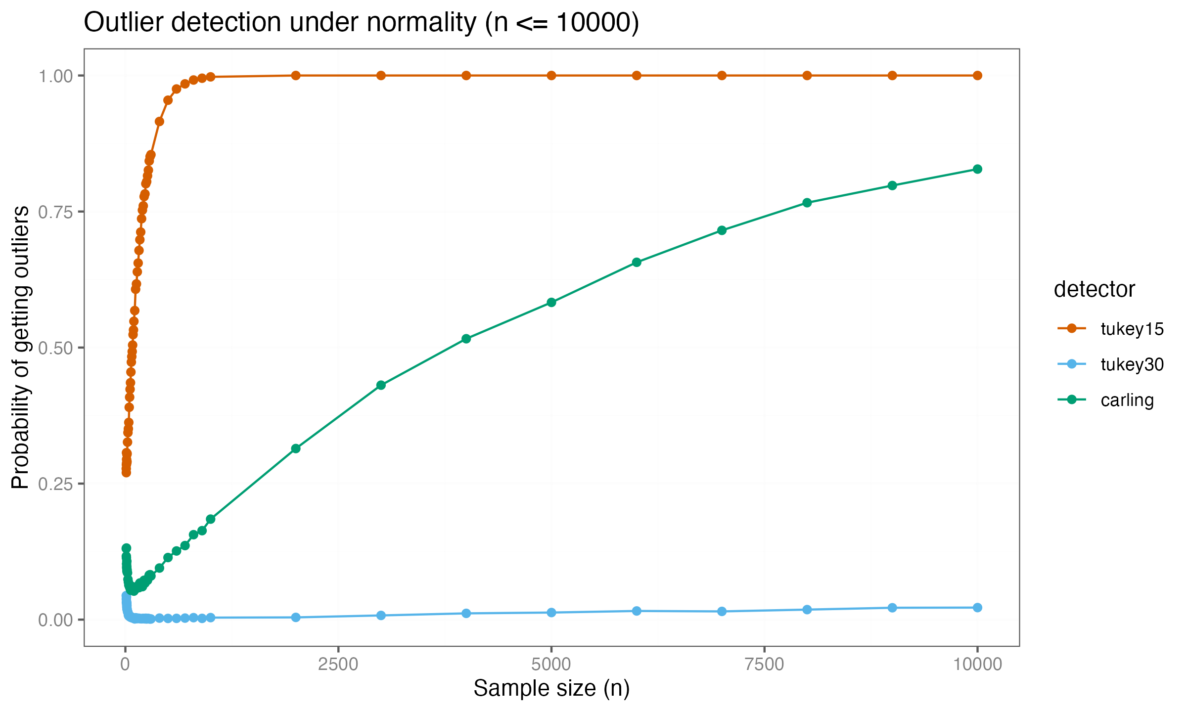
Carling’s method now shows convergence toward a detection rate of $1.0$, indicating that it eventually classifies all values as outliers for sufficiently large samples. The $k = 3.0$ threshold remains near zero at this scale.

Extending the simulation to $n \leq 100\,000$:

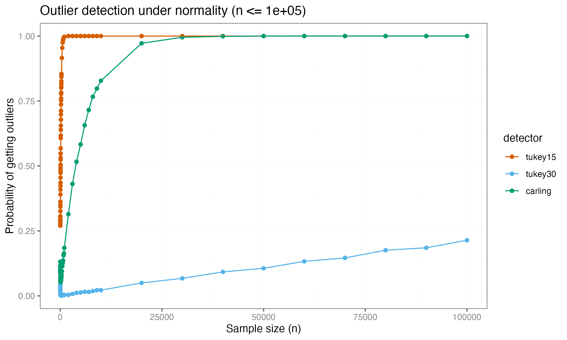
The $k = 3.0$ threshold also begins increasing for very large samples, though it remains lower than Carling’s method. These extended simulations show that asymptotic behavior requires examination across a wide range of sample sizes, as patterns that appear stable at moderate scales can change substantially as $n$ grows.

Analytical evaluation

The detection rate measured in the simulation represents the probability that at least one value in a sample gets classified as an outlier. This section develops asymptotic approximations for these rates and examines where they accurately describe the simulation results.

Asymptotic detection rate formula

For large samples, the sample quartiles converge to their population values. For the standard normal distribution, $Q_1 \approx -0.6745$ and $Q_3 \approx 0.6745$, giving an interquartile range of approximately $1.349$. The Tukey fences stabilize at $\pm(0.6745 + k \cdot 1.349)$ standard deviations from the mean.

Under this asymptotic approximation, the probability that a single observation falls outside these fences is:

$$ p(k) = 2 \cdot \left(1 - \Phi(0.6745 + 1.349k)\right), $$

where $\Phi$ is the standard normal cumulative distribution function.

The probability that at least one value in a sample of size $n$ gets detected as an outlier is:

$$ P_n(k) = 1 - (1 - p(k))^n = 1 - \left(1 - 2\left(1 - \Phi(0.6745 + 1.349k)\right)\right)^n. $$

This formula treats the fences as fixed at their population values, which holds only asymptotically. For small samples, the sample quartiles remain random variables with substantial variance, causing the actual detection rates to deviate from this approximation.

Fixed threshold methods

For the $k = 1.5$ threshold, the fence value is $0.6745 + 1.349 \cdot 1.5 = 2.698$ standard deviations, giving:

$$ P_n(1.5) = 1 - \left(1 - 2(1 - \Phi(2.698))\right)^n \approx 1 - (0.993)^n. $$

This formula shows rapid convergence to perfect detection. At $n = 1000$, the theoretical rate is $0.9991$, closely matching the simulated value of $0.9975$.

For the $k = 3.0$ threshold, the fence value is $0.6745 + 1.349 \cdot 3.0 = 4.721$ standard deviations, giving:

$$ P_n(3.0) = 1 - \left(1 - 2(1 - \Phi(4.721))\right)^n \approx 1 - (0.9999976)^n. $$

The extremely small per-point probability $(p(3.0) \approx 2.4 \times 10^{-6})$ means the detection rate grows slowly. At $n = 1000$, the theoretical rate is $0.0024$, consistent with the simulated value of $0.0037$. Even at $n = 100\,000$, the rate remains approximately $0.21$.

Carling’s adaptive method

For Carling’s method, $k$ depends on sample size:

$$ k(n) = \frac{17.63n - 23.64}{7.74n - 3.71}. $$

As $n$ increases, $k(n)$ approaches $17.63/7.74 \approx 2.277$. The fence value converges to $0.6745 + 1.349 \cdot 2.277 = 3.747$ standard deviations, giving:

$$ P_n(\text{Carling}) \approx 1 - \left(1 - 2(1 - \Phi(3.747))\right)^n \approx 1 - (0.999822)^n. $$

For finite $n$, the exact value requires using $k(n)$ rather than the asymptotic limit. At $n = 1000$, the theoretical rate is $0.163$, matching the simulated value of $0.1847$. At $n = 10\,000$, the rate reaches $0.828$, and by $n = 30\,000$, it exceeds $0.995$.

Comparison and accuracy

These formulas explain the convergence patterns observed in the simulation for large samples. All three methods eventually reach perfect detection (rate $\to 1$) as $n \to \infty$, but convergence speed differs by orders of magnitude. The asymptotic per-point probabilities determine this speed: $k = 1.5$ has $p \approx 0.007$, Carling has $p \approx 0.000178$, and $k = 3.0$ has $p \approx 0.0000024$.

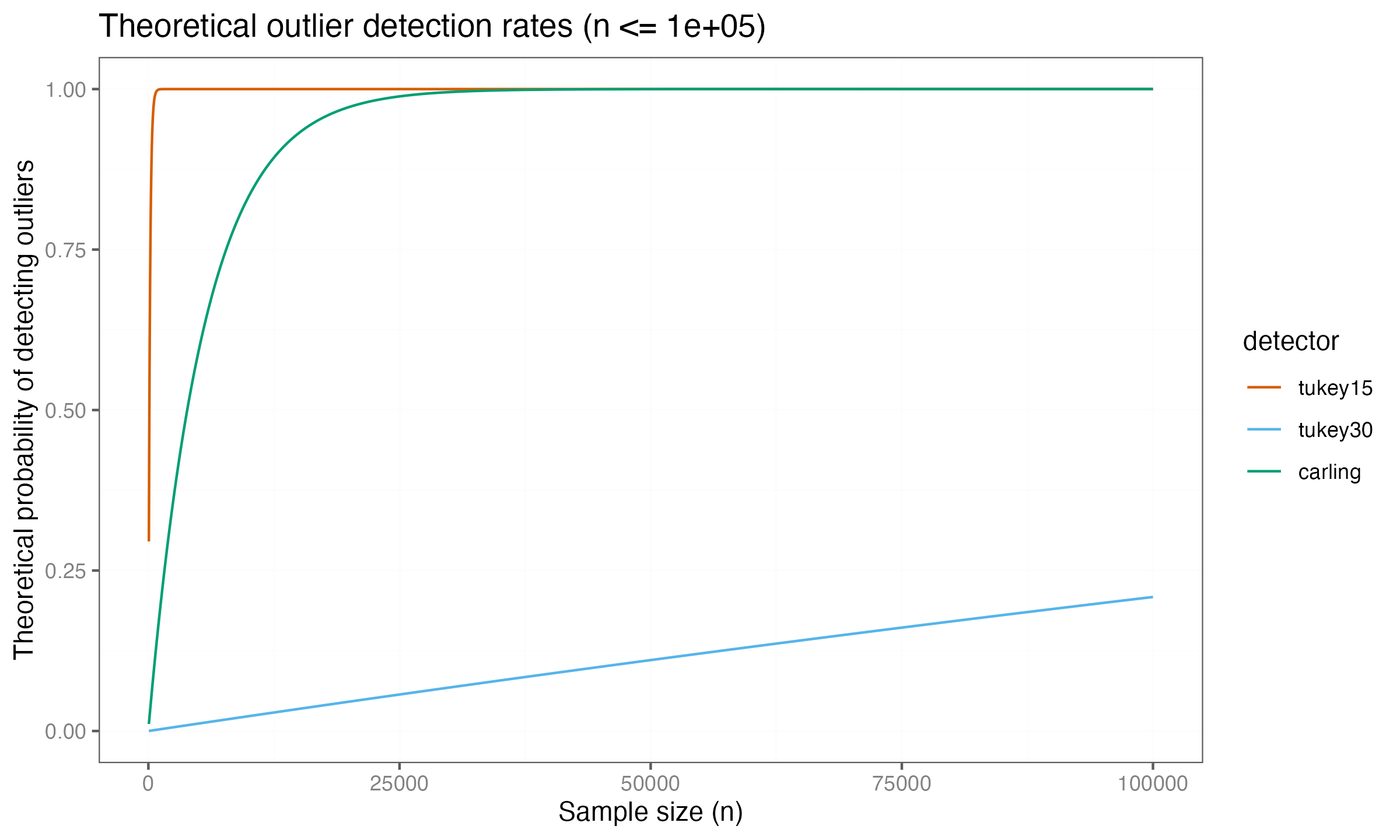
The theoretical curves show the full range of behavior across sample sizes. For large samples ($n \geq 1000$), the asymptotic approximation becomes accurate across all three methods, with theoretical curves closely tracking the simulation results. However, substantial discrepancies appear for smaller samples.

At $n = 10$, the asymptotic formula predicts $P_{10}(1.5) \approx 0.068$, while the simulation shows $0.277$, indicating the formula underestimates by a factor of four. This discrepancy occurs because small-sample quartiles have high variance. The sample quartiles do not reliably estimate the population quartiles for small $n$, and the fence positions fluctuate substantially across samples. When fences happen to fall closer to the center of the data than the asymptotic position, detection rates increase above the asymptotic prediction.

The theoretical curves become reasonably accurate for $n \geq 50$ and highly accurate for $n \geq 1000$, confirming that the formulas correctly capture the long-run behavior. These detection rate formulas reveal that all methods become increasingly sensitive to deviations from normality as sample size grows, eventually flagging observations that would be considered typical under the normal distribution.

Acknowledgement

Thanks to Pavel Gurikov (Hamburg University of Technology) for spotting the mistake in the previous blog post.