A single outlier could completely distort your Cohen's d value
Cohen’s d is a popular way to estimate the effect size between two samples. It works excellent for perfectly normal distributions. Usually, people think that slight deviations from normality shouldn’t produce a noticeable impact on the result. Unfortunately, it’s not always true. In fact, a single outlier value can completely distort the result even in large samples.
In this post, I will present some illustrations for this problem and will show how to fix it.
Cohen’s d
First of all, let’s recall the definition of Cohen’s d. For two samples $x = \{ x_1, x_2, \ldots, x_n \}$ and $y = \{ y_1, y_2, \ldots, y_n \}$, the Cohen’s d is defined as follows ([Cohen1988]):
$$ d_{xy} = \frac{\overline{y}-\overline{x}}{s_{xy}} $$where $s_{xy}$ is the pooled standard deviation:
$$ s_{xy} = \sqrt{\frac{(n_x - 1) s^2_x + (n_y - 1) s^2_y}{n_x + n_y - 2}}. $$There is a rule of thumb that is widely used to interpret Cohen’s d value:
| d | Effect |
|---|---|
| 0.2 | Small |
| 0.5 | Medium |
| 0.8 | Large |
E.g., if $d_{xy} < 0.2$, we can say that the difference between $x$ and $y$ is small. If $d_{xy} > 0.8$, the difference is large
The problem
Now we are going to discuss a simple example that demonstrates the effect of a single outlier. Let’s consider the two following small samples:
$$ x = \{ -1.4,\; -1,\; -0.2,\; 0,\; 0.2,\; 1,\; 1.4 \} \quad \big( \overline{x} = 0,\; s_x = 1 \big), $$$$ y = \{ -0.4,\; 0,\; 0.8,\; 1,\; 1.2,\; 2,\; 2.4 \} \quad \big( \overline{y} = 0,\; s_y = 1 \big). $$Thus, the Cohen’s d equals $1$:
$$ d_{xy} = \frac{\overline{y}-\overline{x}}{s_{xy}} = \frac{1 - 0}{1} = 1. $$We can see that $d_{xy}$ describes a large effect (because it’s larger than 0.8 which is the large effect threshold).
Now let’s replace the last element of $y$ with a high outlier and build a new sample $z$:
$$ z = \{ -0.4,\; 0,\; 0.8,\; 1,\; 1.2,\; 2,\; 100 \} \quad \big( \overline{z} \approx 14.08,\; s_{z} \approx 37.89 \big). $$Since the mean value has been significantly increased ($\overline{z} \approx 14.08 \gg \overline{y} = 0$), we could expect that the Cohen’s d value should be increased as well. However, we observe an opposite situation because of the increased pooled standard deviation:
$$ s_{xz} = \sqrt{\frac{(n_x - 1) s^2_x + (n_z - 1) s^2_z}{n_x + n_z - 2}} = \sqrt{\frac{6\cdot 1^2 + 6\cdot 37.89^2}{12}} \approx 26.8. $$$$ d_{xz} = \frac{\overline{z}-\overline{x}}{s_{xz}} \approx \frac{14.08}{26.8} \approx 0.53. $$As we can see, this outlier spoiled our conclusion. Now, the Cohen’s d equals 0.53 (medium effect) instead of 1.0 (large effect). Technically, the result is correct (because the standard deviation of $z$ is huge), but it doesn’t properly describe the actual difference between $x$ and $y$.
Here you could say that the size of the considered samples is too small, it’s not enough to get a reasonable Cohen’s d value. OK, let’s see what kind of situation we get on larger samples.
Numerical simulations
Let’s conduct the following simulation:
- Generate random sample $x = \{x_1, \ldots, x_n \}$ from $\mathcal{N}(0, 1^2)$.
- Generate random sample $y = \{y_1, \ldots, y_n \}$ from $\mathcal{N}(1, 1^2)$ and replace $y_n$ with $y_n = 100$.
- Calculate the Cohen’s d value between $x$ and $y$.
- Repeat steps previous three steps 1000 times.
- Build a distribution based on 1000 collected Cohen’s d values.
Below you can see corresponding density plots (KDE, normal kernel, Sheather & Jones) for $n = 50$, $n = 500$, and $n = 1000$.
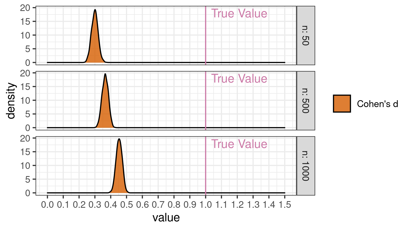
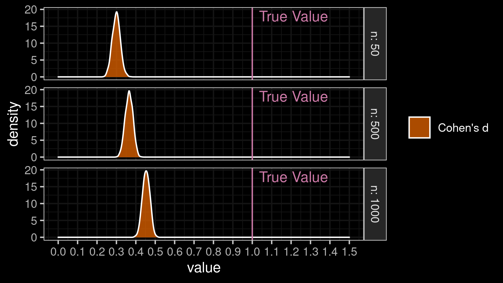
In these simulation, we got the following results:
- $n=50$: all Cohen’s d values are inside $[0.23; 0.37]$
- $n=500$: all Cohen’s d values are inside $[0.30; 0.43]$
- $n=1000$: all Cohen’s d values are inside $[0.39; 0.51]$
As you can see, instead of the expected large effect ($d = 1$), we constantly get small or medium effect ($d < 0.52$). Even when $n = 1000$, a single extreme number could completely distort the result.
So, how to solve this problem?
The solution
In one of the previous posts, I described a nonparametric effect size estimator which is consistent with Cohen’s d. Here is a quick definition:
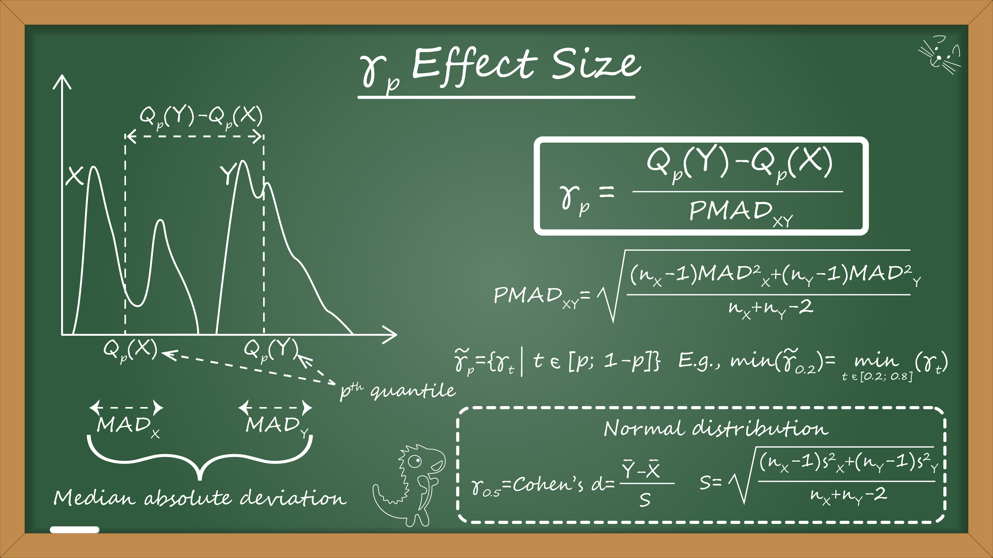
The effect size $\gamma_p$ can be estimated as follows:
$$ \gamma_p = \frac{Q_p(y) - Q_p(x)}{\mathcal{PMAD}_{xy}}, $$where $\mathcal{PMAD}_{xy}$ is the pooled median absolute deviation:
$$ \mathcal{PMAD}_{xy} = \sqrt{\frac{(n_y - 1) \mathcal{MAD}^2_y + (n_y - 1) \mathcal{MAD}^2_y}{n_x + n_y - 2}}. $$In this post, we are going to apply it only for the median (we need only $\gamma_{0.5}$).
In order to improve the accuracy, we use the Harrell-Davis quantile estimator (
A new distribution-free quantile estimator
By Frank E Harrell, C E Davis
·
1982harrell1982)
to estimate the median ($Q_{0.5}$) and the median absolute deviation ($\mathcal{MAD}_x$, $\mathcal{MAD}_y$).
The consistency constant $C$ for $\mathcal{MAD}$ equals $1.4826$, which makes $\mathcal{MAD}$ a consistent estimator for the standard deviation estimation.
Thus, in the case of the normal distribution, $\gamma_p$ could be used as a good approximation of the Cohen’s d. In this case of non-normal distribution, it provides a robust and stable alternative to the Cohen’s d.
Let’s repeat the above simulation with outliers and build corresponding density plots for $\gamma_{0.5}$:
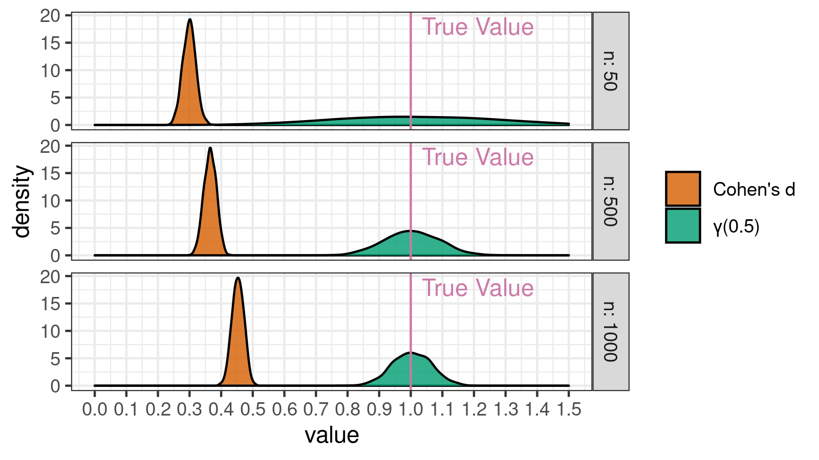
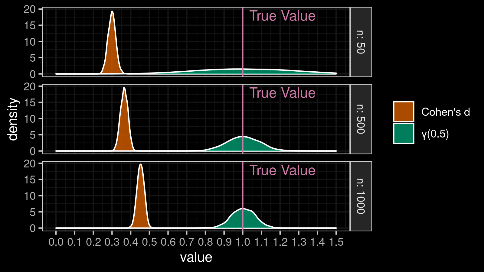
As you can see, a single outlier couldn’t spoil the $\gamma_{0.5}$ values. The obtained effect size values are normally distributed around $1.0$, which is the true effect size value.
Conclusion
The $\gamma_p$ effect size is a good alternative for Cohen’s d. For the normal distributions, it works similar to Cohen’s d. $\gamma_p$ based on two robust metrics (the Harrell-Davis powered medians and median absolution deviations) instead of non-robust metrics in the original Cohen’s d equation (the mean and the standard deviation). Thus $\gamma_p$ is also robust and works well even when we observe deviations from normality. In the case of non-normal distributions, it allows comparing individual quantiles instead of focusing only on the central tendency like the mean or the median.
References
- [Cohen1988]
Cohen, Jacob. (1988). Statistical Power Analysis for the Behavioral Sciences. New York, NY: Routledge Academic - [Harrell1982]
Harrell, F.E. and Davis, C.E., 1982. “A new distribution-free quantile estimator.” Biometrika, 69(3), pp.635-640.
https://pdfs.semanticscholar.org/1a48/9bb74293753023c5bb6bff8e41e8fe68060f.pdf