Comparing distribution quantiles using gamma effect size
There are several ways to describe the difference between two distributions. Here are a few examples:
- Effect sizes based on differences between means (e.g., Cohen’s d, Glass’ Δ, Hedges’ g)
- The shift and ration functions that estimate differences between matched quantiles.
In one of the previous post, I described the gamma effect size which is defined not for the mean but for quantiles. In this post, I want to share a few case studies that demonstrate how the suggested metric combines the advantages of the above approaches.
Case Study 1: Effect size and multimodality
Let’s consider two samples $x$ and $y$ from distributions of the following form:
$$ x \in \textrm{Mixture}(\mathcal{N}(110, 1^2), \mathcal{N}(120, 1^2)) $$$$ y \in \textrm{Mixture}(\mathcal{N}(100, 1^2), \mathcal{N}(130, 1^2)) $$Each distribution is a mixture of two normal distributions. The only difference between them is the location of modes:

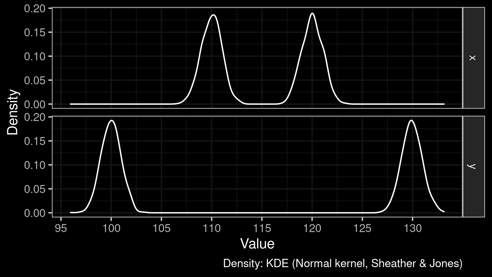
If we compare $x$ and $y$ using a central tendency like the mean or the median, we get zero. The value of the mean and the median for $x$ and $y$ is the same; it equals $115$.
However, if we compare these samples using the $\gamma_p$ effect size, we get an interesting chart:
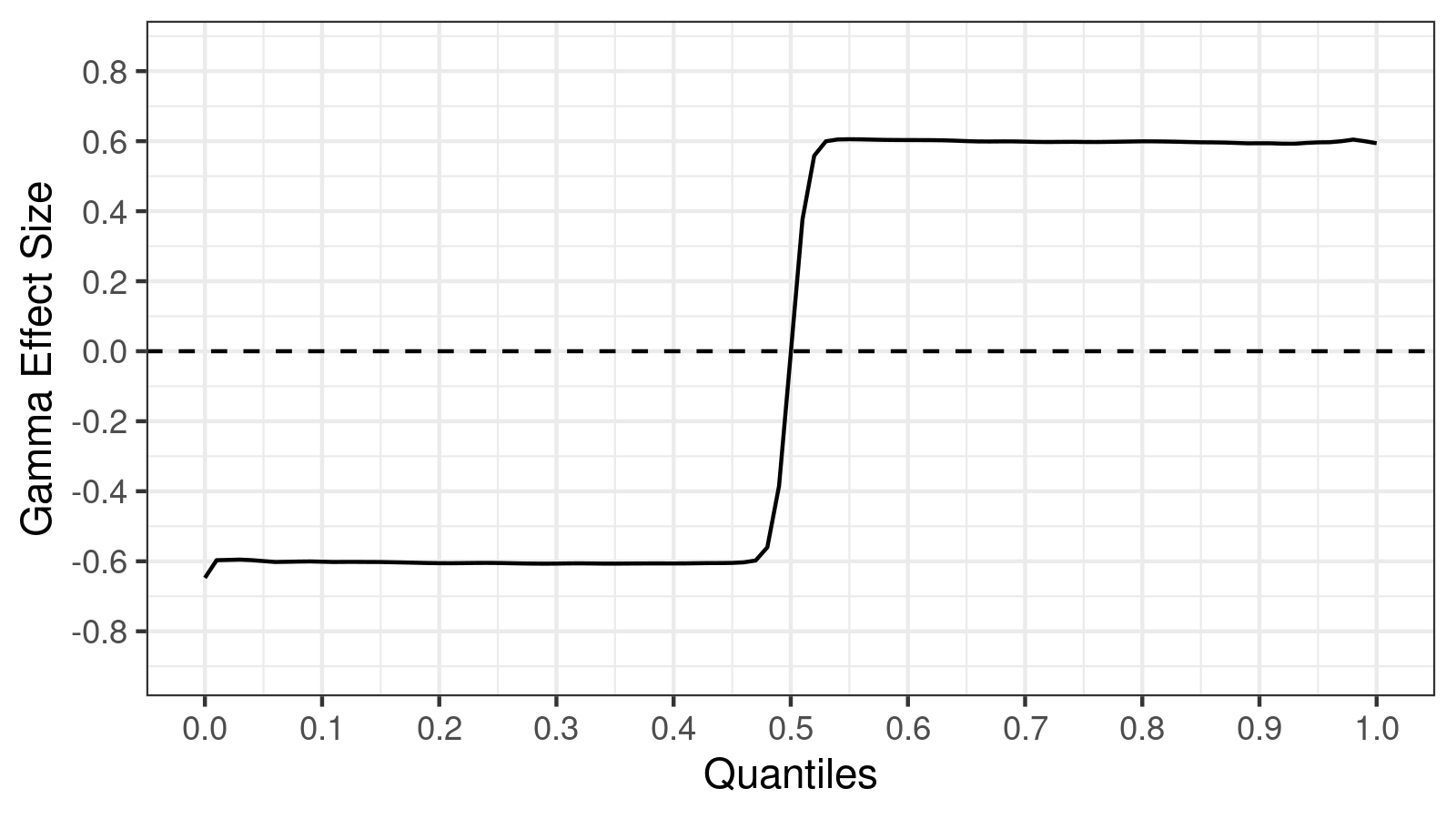

Whereas the difference between medians is zero, the distributions are not the same at all! All the quantile values except the median were changed. From the above chart, we can conclude that both modes were shifted in opposite directions.
The same kind of analysis of nonparametric distributions can be implemented using the shift and ratio functions. Let’s check out another case study that shows the effect size’s benefits against the shift and ratio.
Case Study 2: Shift and ratio function vs. effect Size function
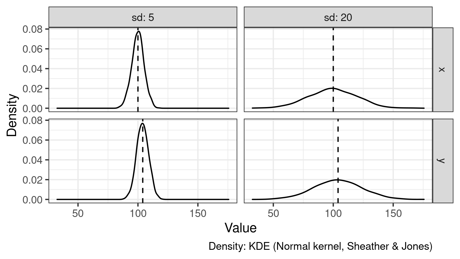
Let’s consider the following two pair of samples:
$$ x^{(1)} \in \mathcal{N}(100, 5^2),\quad y^{(1)} \in \mathcal{N}(104, 5^2) $$$$ x^{(2)} \in \mathcal{N}(100, 20^2),\quad y^{(2)} \in \mathcal{N}(104, 20^2) $$Now all samples are taken from normal distributions with different mean and standard deviation values. Here are their density plots:

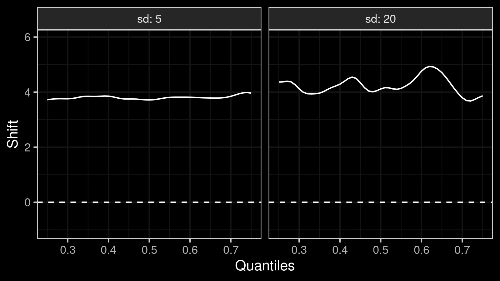
The mean/median difference between $x^{(k)}$ and $y^{(k)}$ is $4$ in both cases. We can see it on the shift function plot:
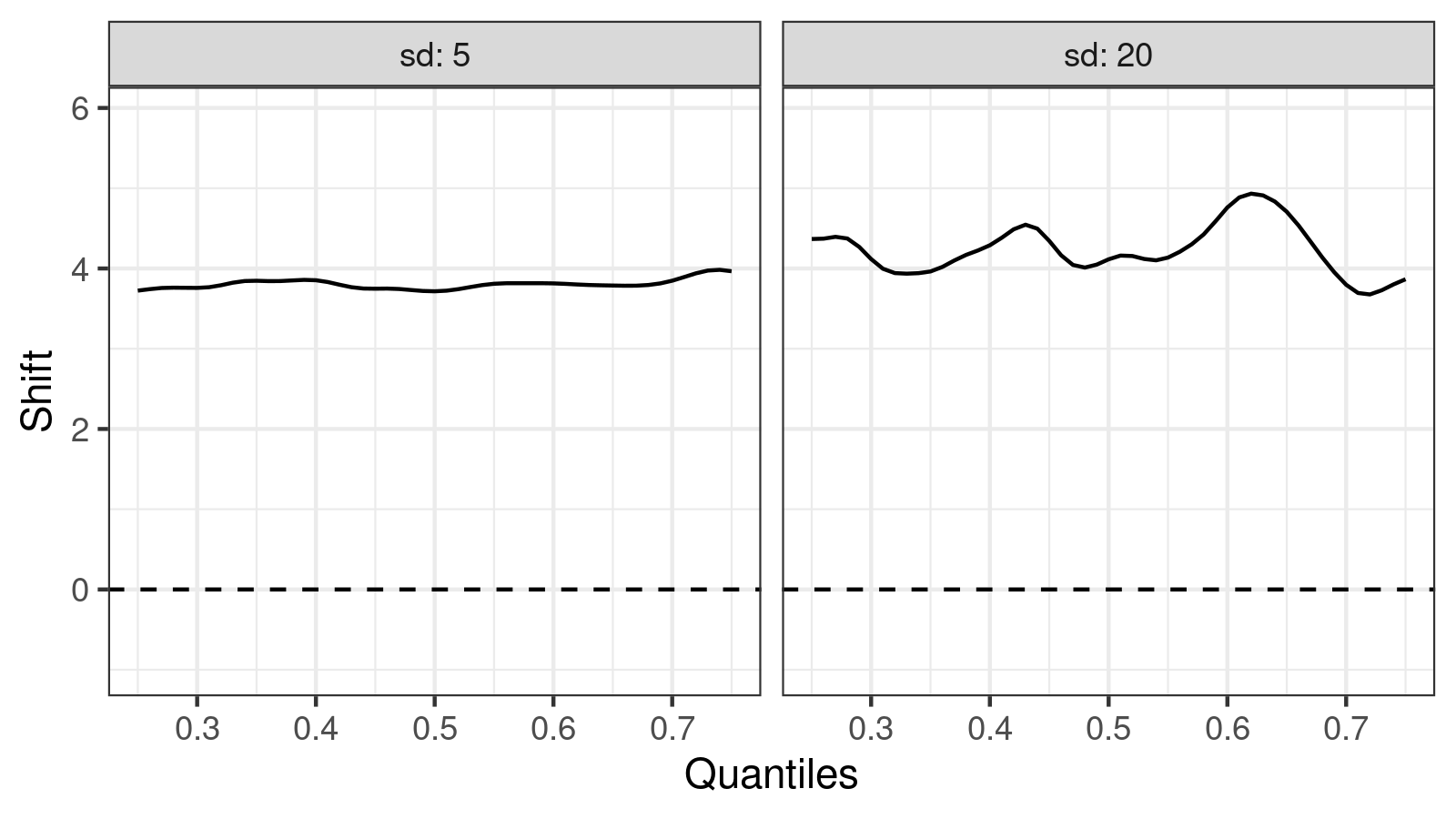
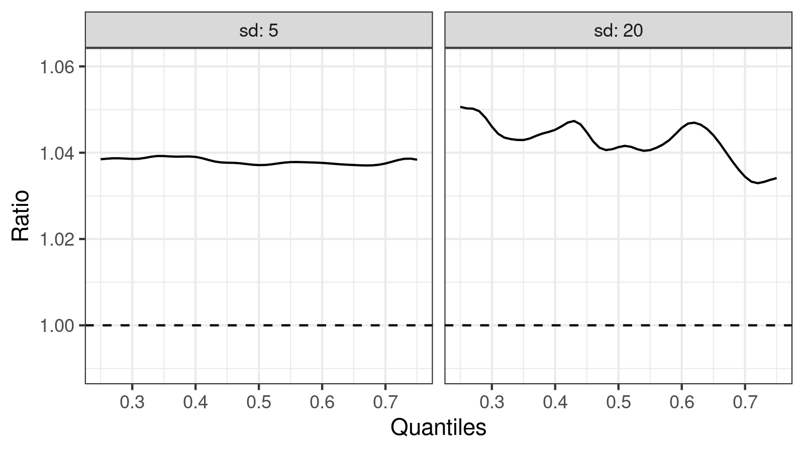
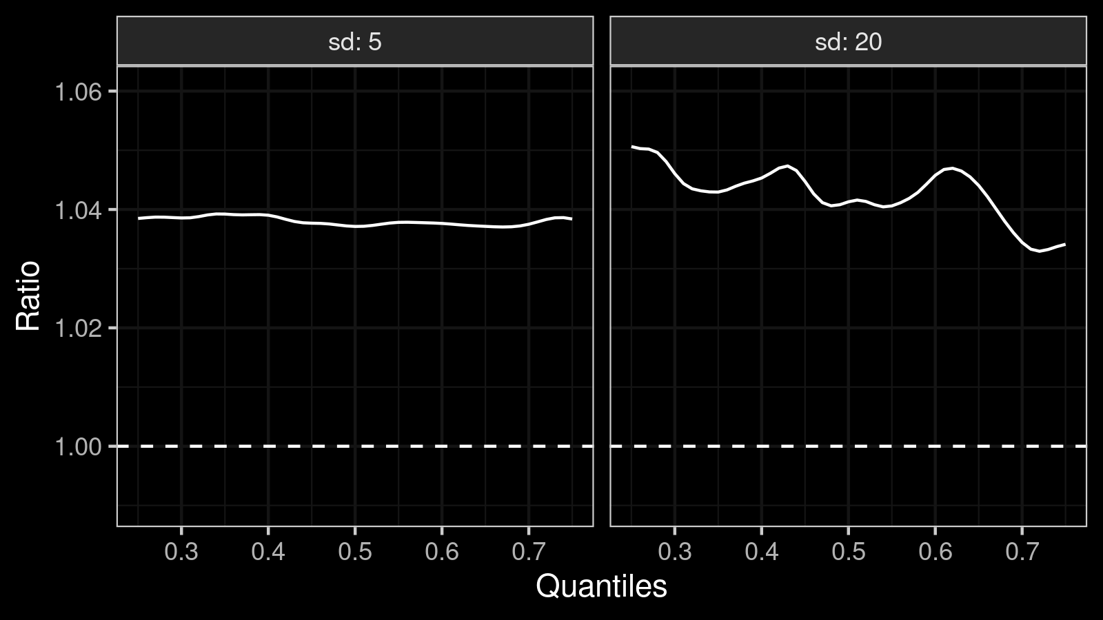
The relative difference is 4%, which is consistent with the ratio function plot:
However, cases are not the same:
- When we compare $x^{(1)}$ and $y^{(1)}$, the standard deviation is $5$. The difference between means/medians is $4$ which is quite large compared to the dispersion.
- When we compare $x^{(2)}$ and $y^{(2)}$, the standard deviation is $20$. The difference between means/medians is also $4$, but it’s not so large compared to the dispersion. While this difference may be statistically significant, it may be practically insignificant.
Now let’s look at the $\gamma$ effect size function plot:
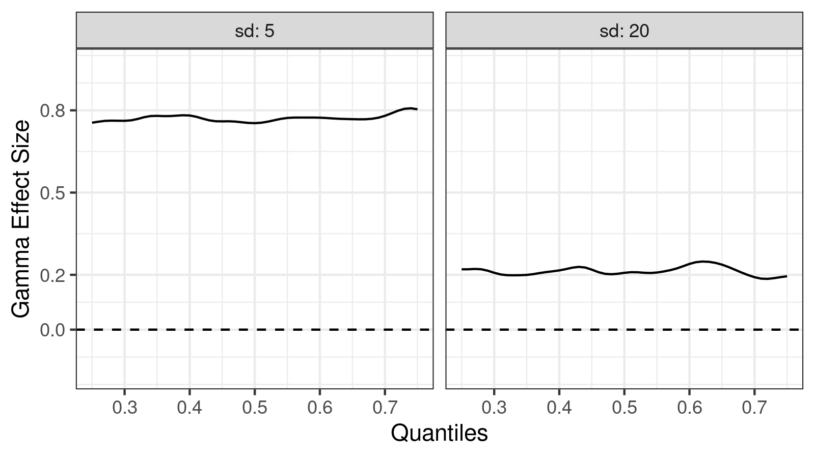
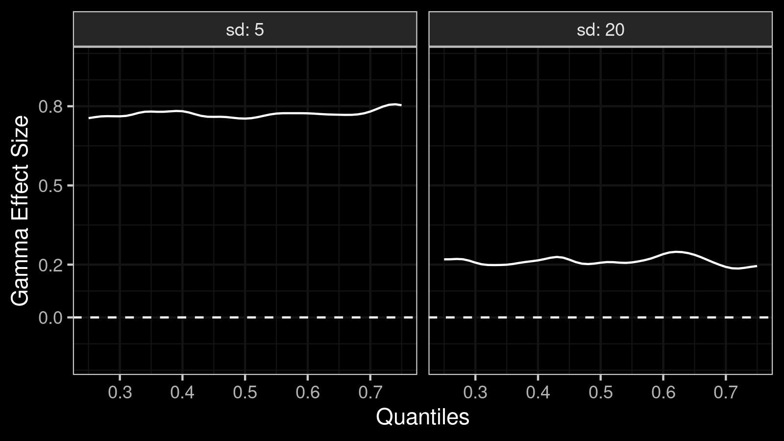
Here we can see that the effect size is large in the first case ($\gamma \approx 0.8$), but it’s small in the second case ($\gamma \approx 0.2$). Such differentiation is one of the main benefits of effect size against the shift and ratio function.
Conclusion
$\gamma$ effect size is a powerful metric that helps you compare distributions. It combines the advantages of the shift and ratio functions (which shows per-quantile differences between distributions) and the effect size (which shows absolute shift normalized by the dispersion).