Case study: Accuracy of the MAD estimation using the Harrell-Davis quantile estimator (Gumbel distribution)

In some of my previous posts, I used the median absolute deviation (MAD) to describe the distribution dispersion:

• DoubleMAD outlier detector based on the Harrell-Davis quantile estimator
• Nonparametric Cohen’s d-consistent effect size
• Quantile absolute deviation: estimating statistical dispersion around quantiles

The MAD estimation depends on the chosen median estimator: we may get different MAD values with different median estimators. To get better accuracy, I always encourage readers to use the Harrell-Davis quantile estimator instead of the classic Type 7 quantile estimator.

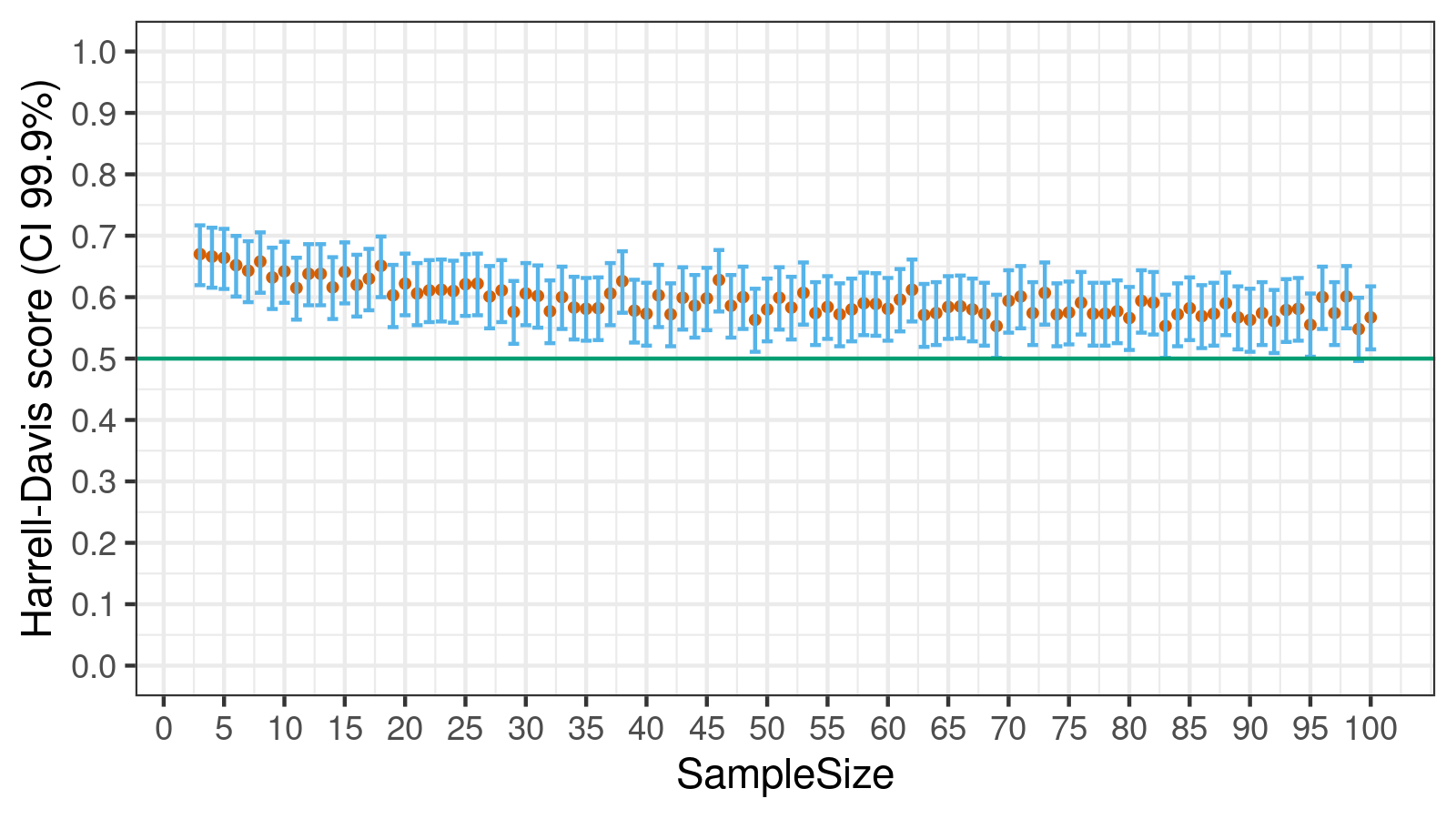
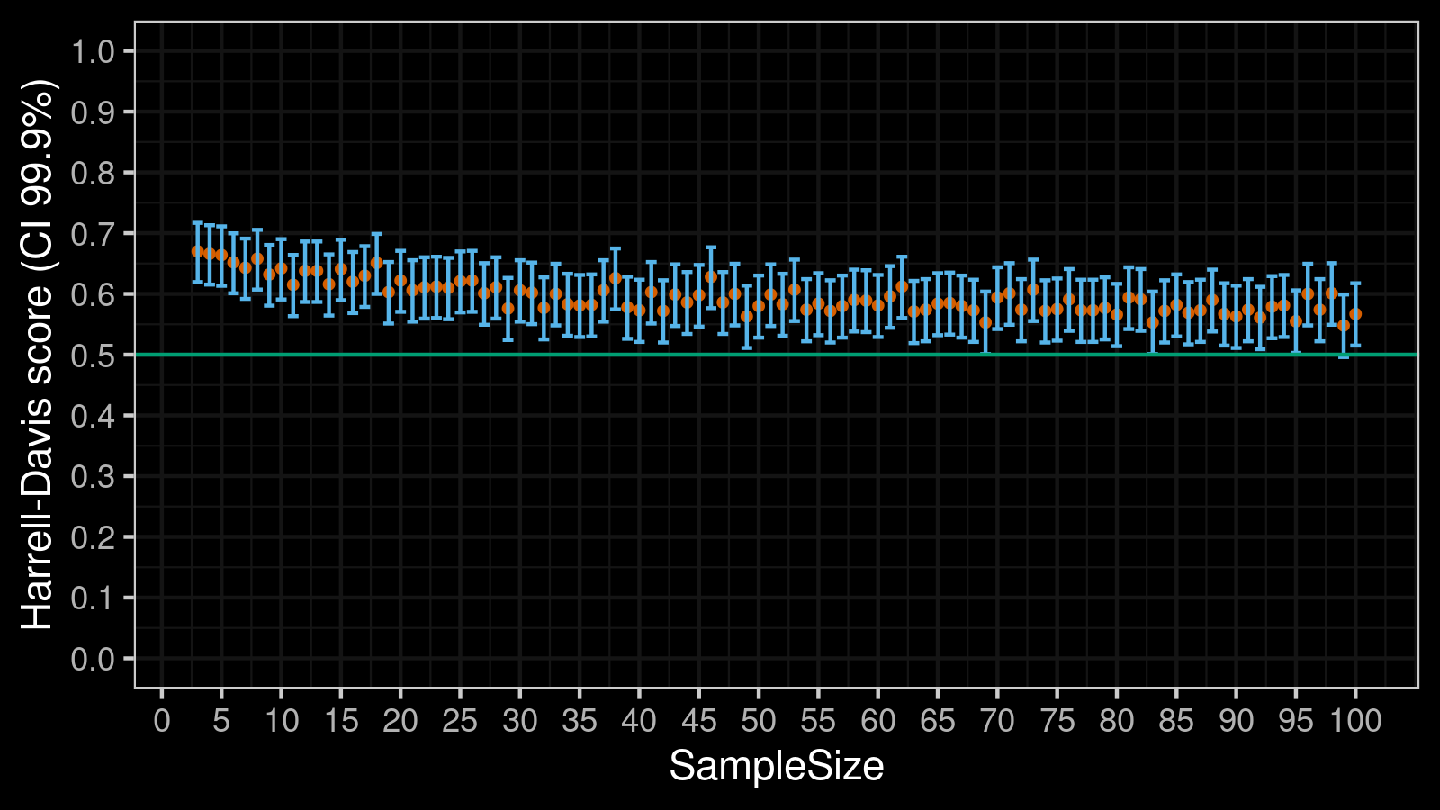
In this case study, I decided to compare these two quantile estimators using the Gumbel distribution (it’s a good model for slightly right-skewed distributions). According to the performed Monte Carlo simulation, the Harrell-Davis quantile estimator always has better accuracy:

The case study

We are going to calculate the median absolute deviation (with the consistency constant = $1$):

We estimate the median using two quantile estimators:

• The Type 7 quantile estimator
  It’s the most popular quantile estimator which is used by default in R, Julia, NumPy, Excel (PERCENTILE, PERCENTILE.INC), Python (inclusive method). We call it “Type 7” according to notation from hyndman1996, where Rob J. Hyndman and Yanan Fan described nine quantile algorithms which are used in statistical computer packages.
• The Harrell-Davis quantile estimator
  It’s my favorite option in real life because it’s more efficient than classic quantile estimators based on linear interpolation, and it provides more reliable estimations on small samples. This quantile estimator is described in harrell1982.

We take random samples from the Gumbel distribution ($\mu = 0,\; \beta = 1$). The true median absolute deviation is known: 0.767049251325708.

Let’s perform the following Monte Carlo simulation:

• Enumerate different sample sizes from 3 to 60
• Perform 1000 iterations for each sample size
• Generate random sample from the gumbel distribution ($\mu = 0,\; \beta = 1$).
• Estimate the median absolute deviation using two quantile estimators
• Evaluate the absolute error for both estimation
• Calculate the portion of cases (“score”) when the Harrell-Davis quantile estimator provides better MAD estimations than the Type 7 quantile estimator.

You can find an R script with the simulation at the end of this post.

In this case study, we got a statistically significant result that shows the superiority of the Harrell-Davis quantile estimator:

The benefits of the Harrell-Davis quantile estimator are most noticeable on small sample sizes ($\textrm{SampleSize} < 20$).

Density plots

Here are some of the density plots for the absolute errors of the median absolute deviation:

The script

The data set has been generated using the following R script:

library(dplyr)
library(tidyr)
library(Hmisc)
library(evd)

t7mad <- function(x) quantile(abs(x - quantile(x, 0.5)), 0.5)
hdmad <- function(x) hdquantile(abs(x - hdquantile(x, 0.5)), 0.5)

build.df <- function(mad.true, gen, iterations) {
  ns <- 3:100
  df <- data.frame(
    SampleSize = rep(ns, each = iterations),
    Type7 = 0,
    HarrellDavis = 0
  )
  for (i in 1:nrow(df)) {
    x <- gen(df[i, "SampleSize"])
    df[i, "Type7"] <- abs(mad.true - t7mad(x))
    df[i, "HarrellDavis"] <- abs(mad.true - hdmad(x))
  }
  df
}

set.seed(42)
iterations <- 1000
df <- build.df(0.767049251325708, function(n) rgumbel(n), iterations)

stats <- df %>%
  group_by(SampleSize) %>%
  dplyr::summarise(
    score = sum(HarrellDavis < Type7) / iterations,
    low = prop.test(sum(HarrellDavis < Type7), n(), conf.level = 0.999, correct = F)$conf.int[1],
    high = prop.test(sum(HarrellDavis < Type7), n(), conf.level = 0.999, correct = F)$conf.int[2]
    )

References

• [Harrell1982]
  Harrell, F.E. and Davis, C.E., 1982. A new distribution-free quantile estimator. Biometrika, 69(3), pp.635-640.
  https://pdfs.semanticscholar.org/1a48/9bb74293753023c5bb6bff8e41e8fe68060f.pdf
• [Hyndman1996]
  Hyndman, R. J. and Fan, Y. 1996. Sample quantiles in statistical packages, American Statistician 50, 361–365.
  https://doi.org/10.2307/2684934