Improving the efficiency of the Harrell-Davis quantile estimator for special cases using custom winsorizing and trimming strategies

Let’s say we want to estimate the median based on a small sample (3 $\leq n \leq 7$) from a right-skewed heavy-tailed distribution with high statistical efficiency.

The traditional median estimator is the most robust estimator, but it’s not the most efficient one. Typically, the Harrell-Davis quantile estimator provides better efficiency, but it’s not robust (its breakdown point is zero), so it may have worse efficiency in the given case. The winsorized and trimmed modifications of the Harrell-Davis quantile estimator provide a good trade-off between efficiency and robustness, but they require a proper winsorizing/trimming rule. A reasonable choice of such a rule for medium-size samples is based on the highest density interval of the Beta function (as described here). Unfortunately, this approach may be suboptimal for small samples. E.g., if we use the 99% highest density interval to estimate the median, it starts to trim sample values only for $n \geq 8$.

In this post, we are going to discuss custom winsorizing/trimming strategies for special cases of the quantile estimation problem.

Beware of small samples

So, what’s wrong with the small samples from heavy-tailed distributions? There is a high chance to observe an extremely large value in such a sample. As an example, let’s consider the Pareto distribution. Here is the PDF for $\textrm{Pareto}(x_m = 1, \alpha = 1)$:

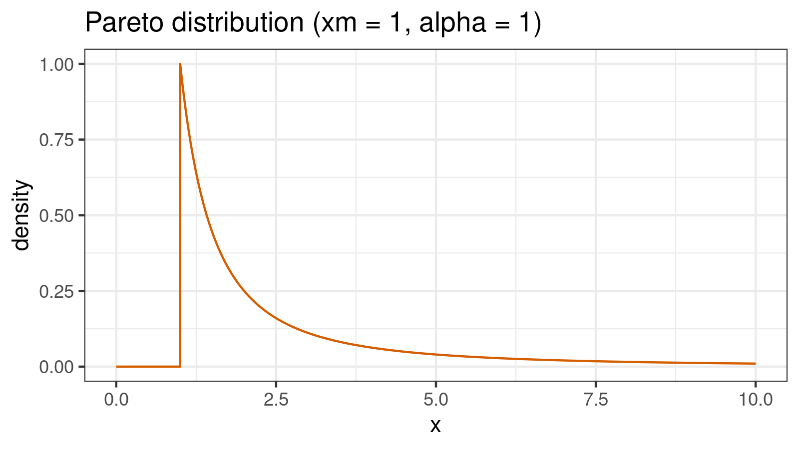
The quantile function for the Pareto distribution is defined as follows:

In our case ($x_m = 1, \alpha = 1$), we have:

Here are some of the quantile values:

q[0.500] = 2
q[0.750] = 4
q[0.900] = 10
q[0.950] = 20
q[0.990] = 100
q[0.999] = 1000

Thus, while the median value is $2$, the value of the $99.9^\textrm{th}$ percentile is 1000. It may look like a small probability, but this impression is deceiving. For example, if we consider 5000 values (or 1000 of 5-element samples), there is a 99.3% chance that at least one of the values is higher than 1000.

The problem of the Harrell-Davis quantile estimator

The Harrell-Davis approach suggests estimating the quantile value as a weighted sum of all sample elements where all weight values are positive. Thus, its breakdown point is zero: a single “extreme” value may “corrupt” the estimation. Let’s say we have the following sample from $\textrm{Pareto}(x_m = 1, \alpha = 1)$:

The traditional median estimator just selects the middle element. In our case, it gives

which is a pretty accurate median estimation. The Harrell-Davis quantile estimator produces a worse estimation:

The Harrell-Davis quantile estimator is a good approach in many cases because it typically provides better efficiency then the traditional one. Unfortunately, in the considered case (small samples form heavy-tailed distribution), its efficiency is quite bad because it’s not robust enough. Let’s try to fix this problem.

Smart winsorizing/trimming

If we want to improve the Harrell-Davis quantile estimator robustness, we can consider its winsorized and trimmed modifications. In one of the previous posts, I described an approach that selects the trimming percentage based on the highest density interval of the corresponding beta function. It works great for medium-size samples, but it’s useless for small samples. If we use the 99% highest density interval to estimate the median, the trimming percentage will be positive only for $n \geq 8$.

In our case, we can consider a custom trimming strategy. Our greatest enemy here is the random extreme values. We want to trim them whenever it’s possible.

Let’s consider a sample $x$ with $n$ elements where all the samples elements are already sorted:

Now let’s discuss how we should trim the samples for different $n$ values:

• $n=3$
  It’s not a good idea to trim $x_2$ because it’s our traditional median estimation. It’s also doesn’t make sense to trim $x_1$ because the considered distribution is right-skewed ($x_1$ is the minimum element of the sample; it has the smallest chance to be “extreme”). Thus, the reasonable decision is to trim $x_3$.
• $n=4$
  The traditional median estimator for samples with even size uses two middle elements. For $n=4$, these elements are $x_2$ and $x_3$, so we don’t want to trim them. It’s still useless to trim $x_1$, so our only option is to trim $x_4$.
• $n=5$
  Here the traditional median estimator uses only $x_3$. So, we can trim two elements: $x_4$ and $x_5$.
• $n=6$
  By analogy, we can trim $x_5$ and $x_6$.
• $n=7$
  Here the traditional median estimator uses only $x_4$. Thus, we can trim three elements: $x_5$, $x_6$, and $x_7$.

This strategy can be described using the following scheme (@ denotes non-trimmed element; x denotes trimmed element; assuming sorted sample):

n = 3: @@x
n = 4: @@@x
n = 5: @@@xx
n = 6: @@@@xx
n = 7: @@@@xxx

It’s time to check how it works.

Numerical simulation

We are going to compare four quantile estimators:

• hf7: the traditional quantile estimator (also known as the Hyndman-Fan Type 7)
• hd: the Harrell-Davis quantile estimator
• whd: the winsorized Harrell-Davis quantile estimator where the winsorized elements are defined according to the scheme from the previous section
• thd: the trimmed Harrell-Davis quantile estimator where the trimmed elements are defined according to the scheme from the previous section

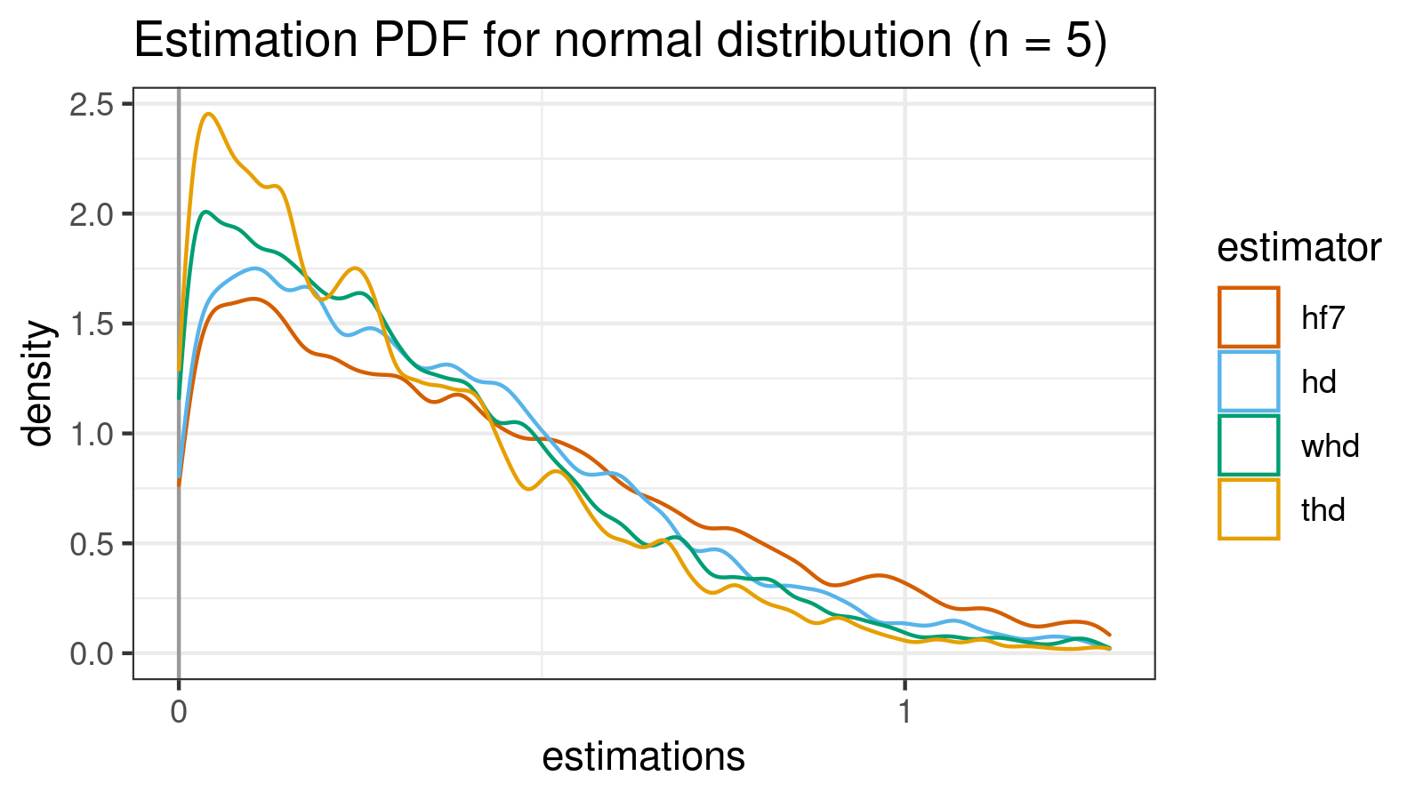
Typically, the estimator efficiency is evaluated using the mean squared error (mse) and the bias. This approach works good for light-tailed error distribution, but it could be misleading for heavy-tailed distribution. Thus, in addition to the classic bias and mse metric, we also consider different percentiles of the absolute values of simulated errors. Also, we are going to draw the PDF of the error distributions. Each error distribution is based on 100'000 random samples.

In this simulation, we are going to estimate the median for the normal distribution (the true median value is $0$) and for $\textrm{Pareto}(x_m = 1, \alpha = 1)$ (the true median value is $2$).

Normal distribution (n = 5)

Let’s start with the normal distribution (which is symmetric and light-tailed) to do a dry-check of our estimators.

 estimator       bias     mse     p25     p50     p75     p90     p95    p99
       hf7 -0.0016329 0.29153 0.16804 0.36103 0.61964 0.89926 1.06836 1.3611
        hd -0.0056730 0.21042 0.14671 0.31081 0.52609 0.74722 0.89905 1.1936
       whd -0.1920940 0.28335 0.17178 0.36076 0.60780 0.87269 1.04119 1.3885
       thd -0.2879419 0.32841 0.18283 0.38710 0.65326 0.94229 1.14017 1.4771

TODO: rewrite As we can see, hf7 and hd give pretty similar results. In this particular case, whd and thd give worse results (but they are still pretty acceptable) It’s an expected situation because our winsorizing/trimming strategy is “overfitted” to the right-skewed case while the actual distribution is symmetric.

Pareto distribution (n = 3)

Now it’s time to check our estimators on the most complicated case: we should guess the median value of $\textrm{Pareto}(x_m = 1, \alpha = 1)$ based only on three elements!

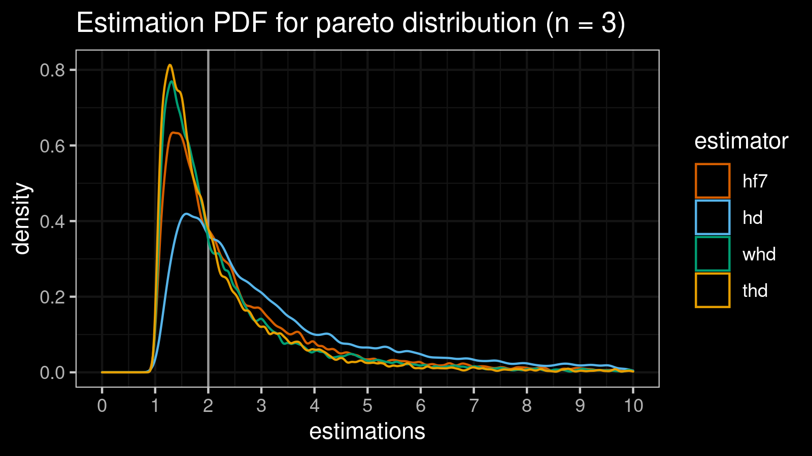
 estimator     bias        mse     p25     p50     p75    p90     p95    p99
       hf7  0.96402     14.093 0.33215 0.63298 1.09961 3.1286  5.4061 15.677
        hd 12.75015 175467.942 0.37914 0.84069 3.02464 8.9115 18.5175 90.129
       whd  0.62981     14.147 0.32802 0.61526 0.89961 2.4955  4.2395 11.140
       thd  0.48012     23.503 0.33245 0.61360 0.88120 1.9543  3.4305  9.819

Expectedly, hd has the worst error values because of its zero breakdown point. Meanwhile, whd and thd have better error values than hf7 (which is our baseline). They are better not only based on the “classic” bias and mse metrics but only based on all the percentile values.

Let’s see what happens for higher $n$ values.

Pareto distribution (n = 4)

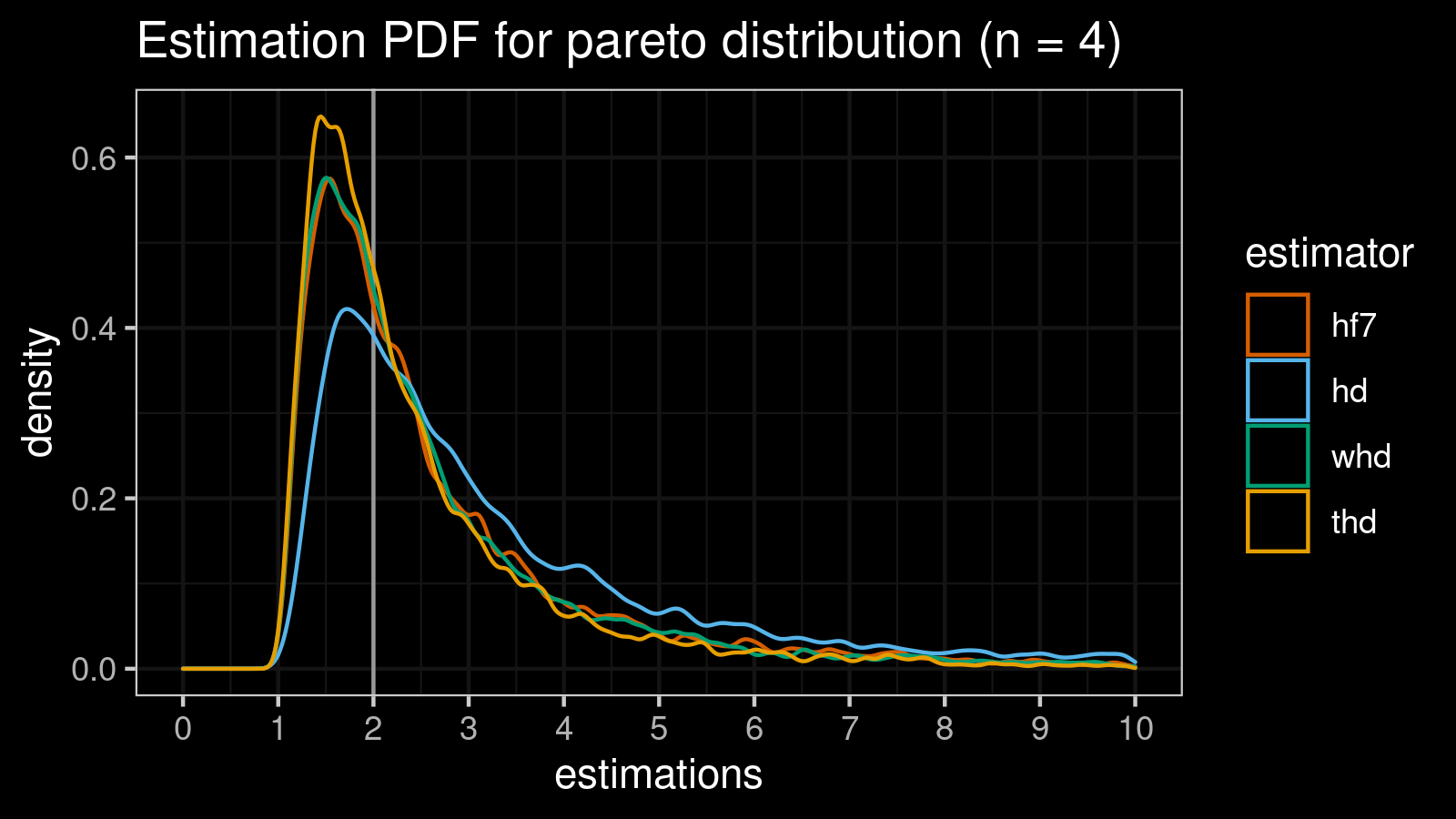
 estimator    bias      mse     p25     p50     p75    p90     p95    p99
       hf7 0.99630   13.376 0.28927 0.58443 1.22370 3.1813  5.1862 12.015
        hd 4.33302 1376.949 0.35408 0.81399 2.56402 6.8722 12.2750 53.703
       whd 0.95874   25.060 0.28729 0.57546 1.12468 2.9193  4.8311 12.190
       thd 0.72518   11.554 0.27726 0.54553 0.91749 2.3926  4.0997 10.723

Pareto distribution (n = 5)

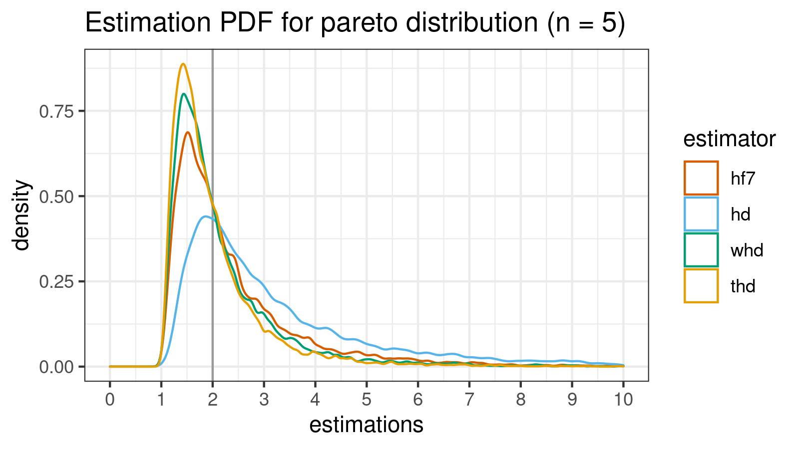
 estimator     bias        mse     p25     p50     p75    p90    p95     p99
       hf7 0.504146     5.2105 0.26675 0.52613 0.87303 2.1065 3.3679  7.2826
        hd 4.396743 22596.2795 0.31288 0.74502 2.24599 5.3275 9.3600 34.9101
       whd 0.231205     2.1152 0.26279 0.50793 0.77450 1.4745 2.4296  5.8547
       thd 0.067092     1.6300 0.26268 0.50467 0.74328 1.1175 1.9506  4.6478

Pareto distribution (n = 6)

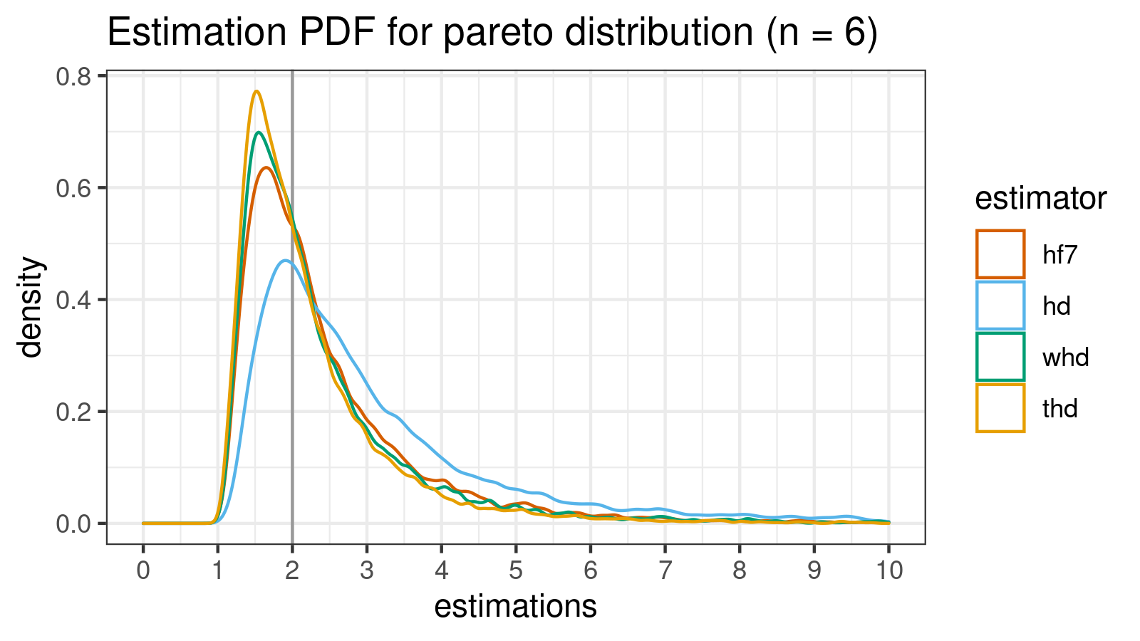
 estimator    bias       mse     p25     p50     p75    p90    p95     p99
       hf7 0.51371    2.5938 0.23690 0.48757 0.86252 2.0152 3.0778  6.4690
        hd 2.46898 1195.1400 0.29120 0.66492 1.78711 4.0332 6.8272 20.9587
       whd 0.42000    2.5518 0.23282 0.47884 0.79029 1.7981 2.8478  6.0907
       thd 0.25985    1.4532 0.23638 0.46981 0.74189 1.4778 2.3190  4.9017

Pareto distribution (n = 7)

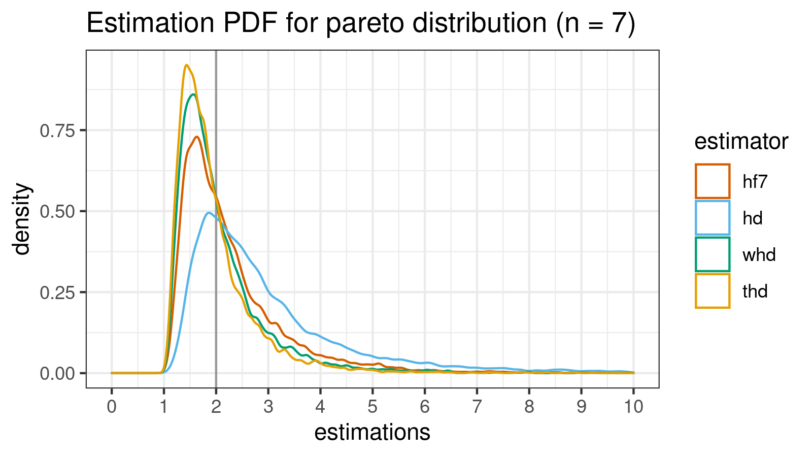
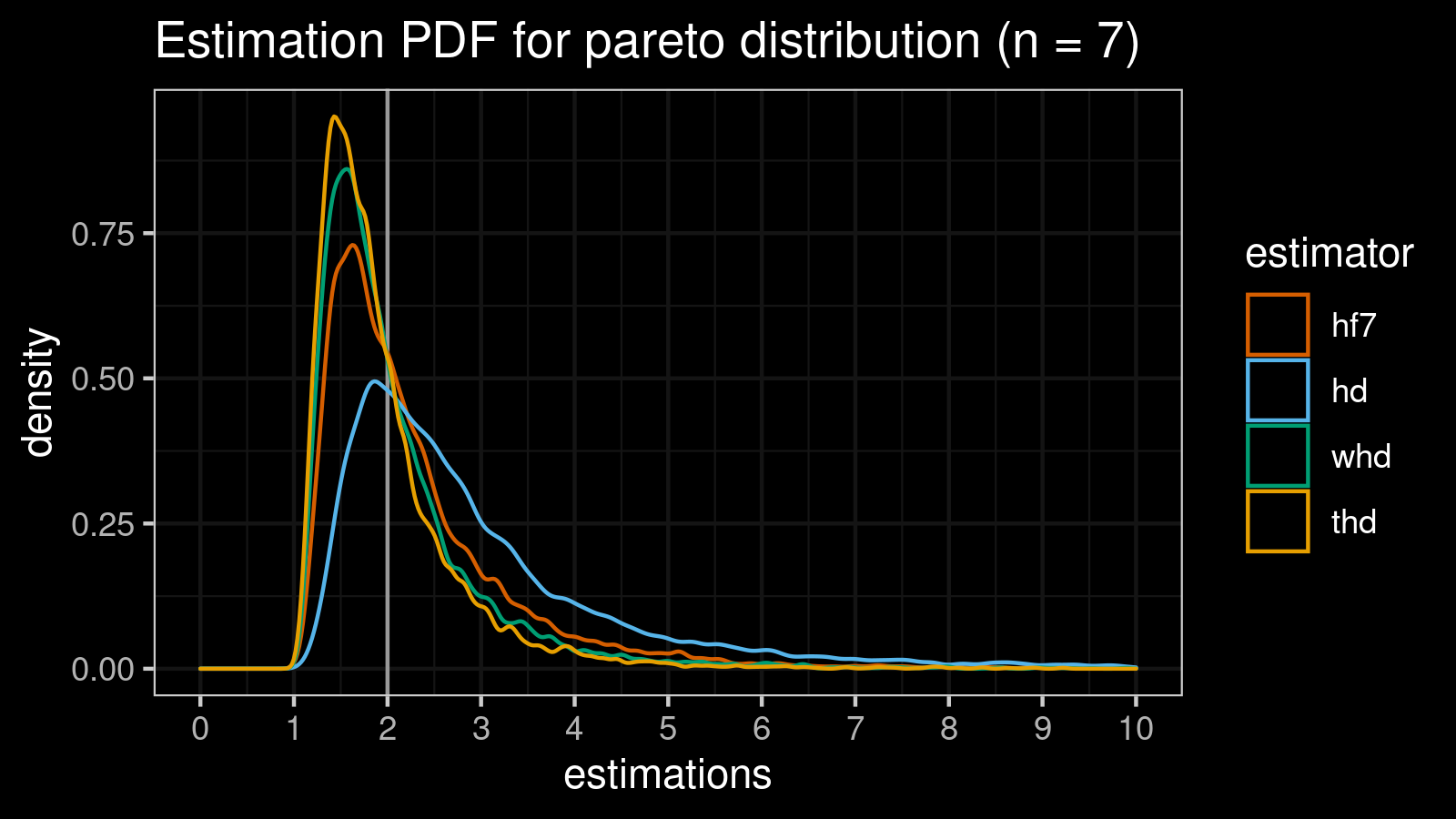
 estimator      bias        mse     p25     p50     p75    p90    p95     p99
       hf7  0.337121    1.85904 0.23519 0.46158 0.75627 1.5838 2.4504  5.3569
        hd  1.975857 1989.76770 0.26722 0.60452 1.52104 3.2602 5.0468 13.5435
       whd  0.082059    0.88772 0.23247 0.44718 0.68616 1.0932 1.7480  3.8571
       thd -0.039714    0.68217 0.23089 0.45429 0.67313 0.8878 1.3837  3.0663

Conclusion

In this post, we performed a numerical simulation that compared the statistical efficiency of the median estimation on small samples from right-skewed heavy-tailed distributions. We compared four quantile estimators: the traditional one (also known as the Hyndman-Fan Type 7), the Harrell-Davis quantile estimator, and its winsorized/trimming modifications that use a custom trimming strategy optimized for the given case. Based on the simulation results, we can conclude that the trimmed modification is the clear winner.