Discrete performance distributions
When we collect software performance measurements, we get a bunch of time intervals. Typically, we tend to interpret time values as continuous values. However, the obtained values are actually discrete due to the limited resolution of our measurement tool. In simple cases, we can treat these discrete values as continuous and get meaningful results. Unfortunately, discretization may produce strange phenomena like pseudo-multimodality or zero dispersion. If we want to set up a reliable system that automatically analyzes such distributions, we should be aware of such problems so we could correctly handle them.
In this post, I want to share a few of discretization problems in real-life performance data sets (based on the Rider performance tests).
General discretization
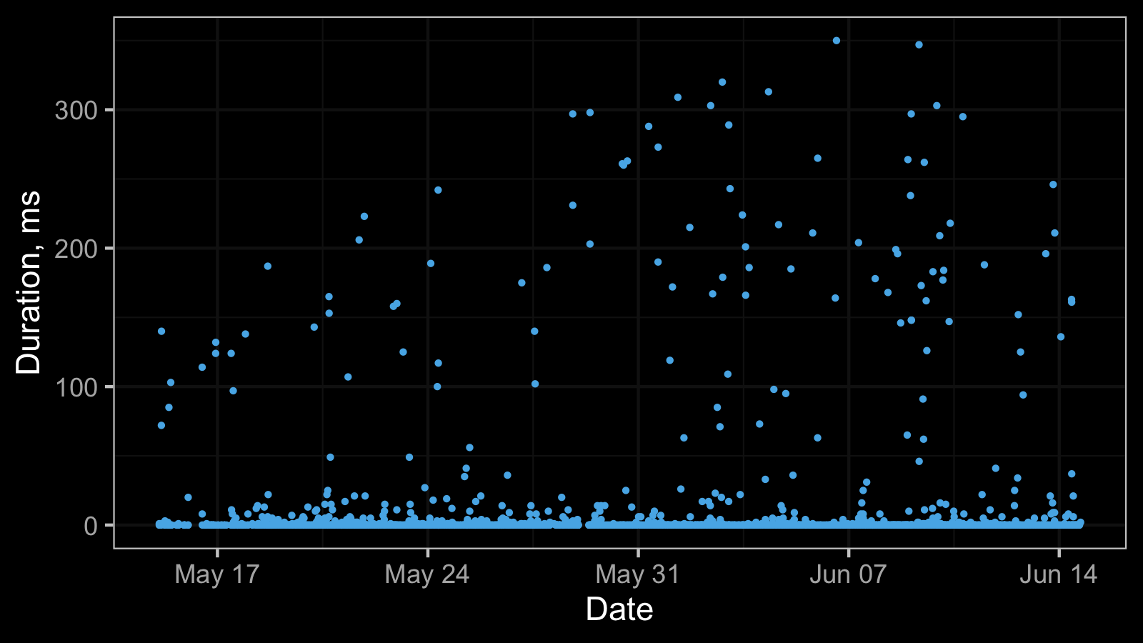
The most simple way to get discretization phenomena is to limit the resolution of your performance measurements to milliseconds. It’s a perfectly legitimate approach when you don’t care about better precision. As a result, we can obtain a timeline plot like this:
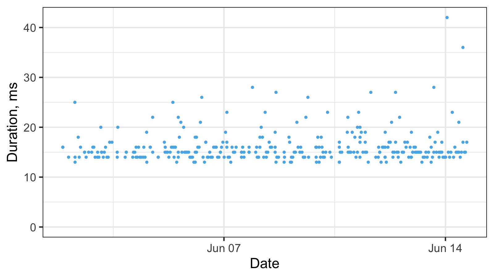
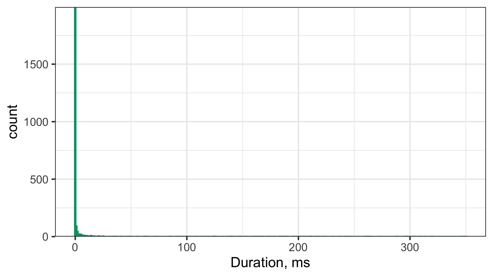
And here is the corresponding histogram (binwidth = 1):

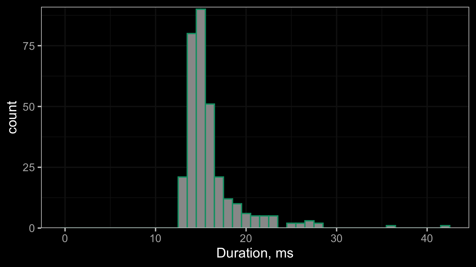
This histogram can be treated as an estimation of the probability mass function of the underlying discrete distribution. However, if we try to treat this distribution as a continuous one and build a density estimation, we can get a corrupted visualization. This problem can be resolved for different kinds of density estimations using jittering (I already blogged about how to do it for the kernel density estimation (KDE) and quantile-respectful density estimation (QRDE)).
Zero median and zero MAD
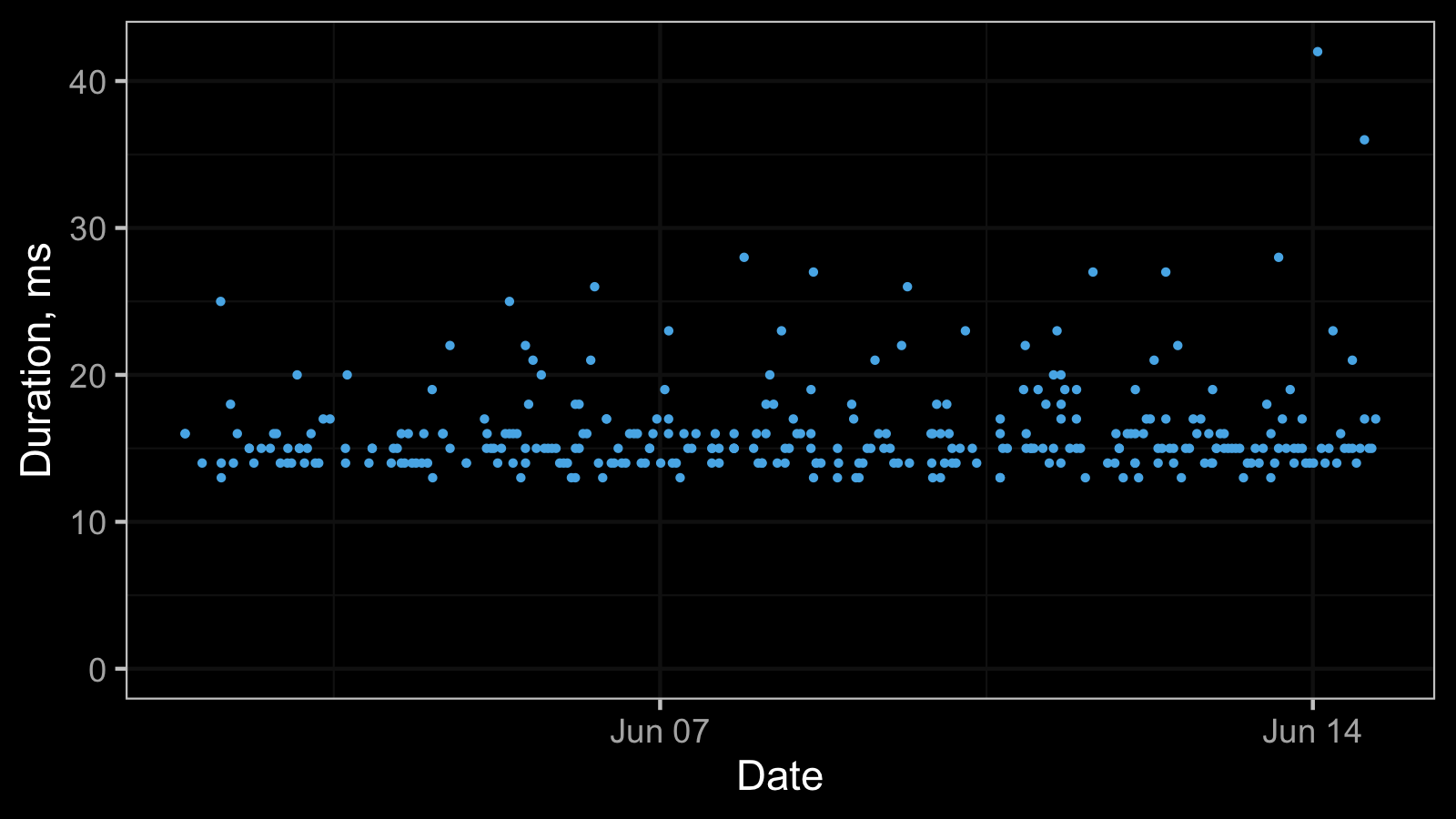
Here is another timeline plot based on real-life performance measurements:
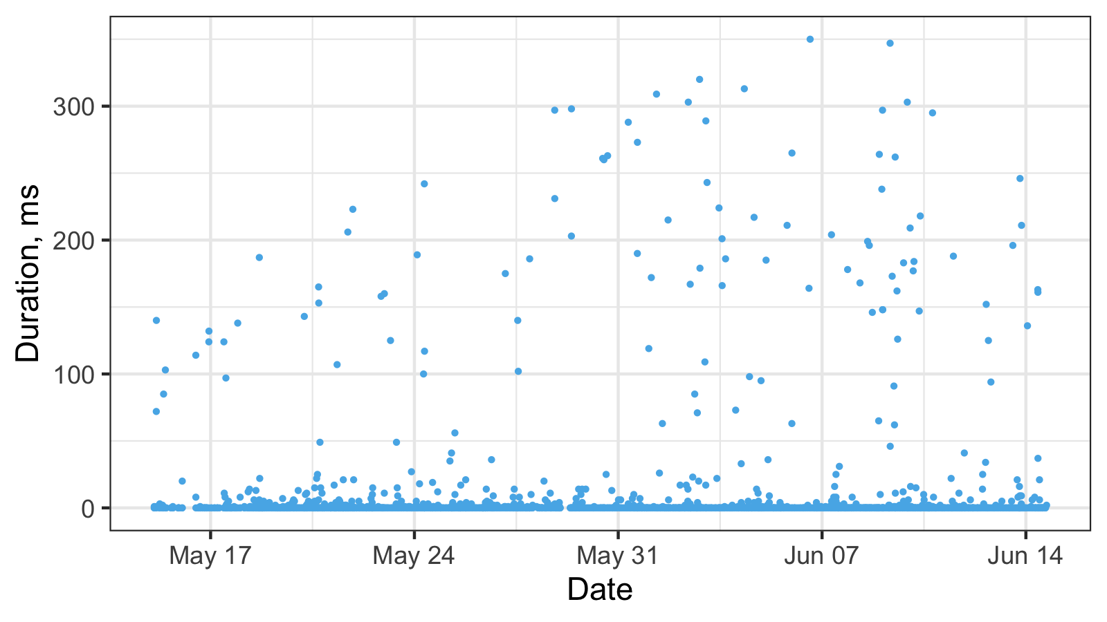
And here is the corresponding histogram:
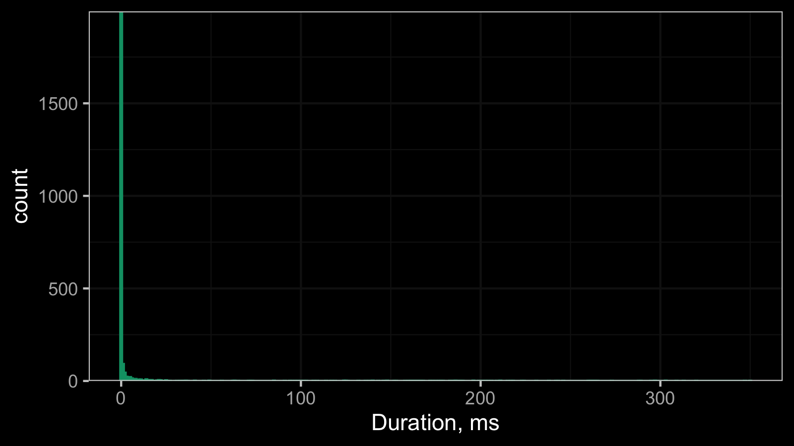
It’s hard to work with such a histogram because of the scale, so here is its raw data:
   0    1    2    3    4    5    6    7    8    9   10   11   12   13   14   15
1996   92   45   23   20   21   14    5   11    5    8    8    3    3    9    5
  16   17   18   19   20   21   22   23   25   26   27   31   33   34   35   36
   3    5    1    1    3    5    4    1    4    1    1    1    1    1    1    2
  37   41   46   49   56   62   63   65   71   72   73   85   91   94   95   97
   1    2    1    2    1    1    2    1    1    1    1    2    1    1    1    1
  98  100  102  103  107  109  114  117  119  124  125  126  132  136  138  140
   1    1    1    1    1    1    1    1    1    2    2    1    1    1    1    2
 143  146  147  148  152  153  158  160  161  162  163  164  165  166  167  168
   1    1    1    2    1    1    1    1    1    1    1    1    1    1    1    1
 172  173  175  177  178  179  183  184  185  186  187  188  189  190  196  199
   1    1    1    1    1    1    1    1    1    2    1    1    1    1    2    1
 201  203  204  206  209  211  215  217  218  223  224  231  238  242  243  246
   1    1    1    1    1    2    1    1    1    1    1    1    1    1    1    1
 260  261  262  263  264  265  273  288  289  295  297  298  303  309  313  320
   1    1    1    1    1    1    1    1    1    1    2    1    2    1    1    1
 347  350
   1    1
These numbers mean the follow: we observed 0ms 1996 times, 1ms 92 times, 2ms 45 times, and so on.
And here are the same set of numbers scaled to percents:
    0     1     2     3     4     5     6     7     8     9    10    11    12
82.68  3.81  1.86  0.95  0.83  0.87  0.58  0.21  0.46  0.21  0.33  0.33  0.12
   13    14    15    16    17    18    19    20    21    22    23    25    26
 0.12  0.37  0.21  0.12  0.21  0.04  0.04  0.12  0.21  0.17  0.04  0.17  0.04
   27    31    33    34    35    36    37    41    46    49    56    62    63
 0.04  0.04  0.04  0.04  0.04  0.08  0.04  0.08  0.04  0.08  0.04  0.04  0.08
   65    71    72    73    85    91    94    95    97    98   100   102   103
 0.04  0.04  0.04  0.04  0.08  0.04  0.04  0.04  0.04  0.04  0.04  0.04  0.04
  107   109   114   117   119   124   125   126   132   136   138   140   143
 0.04  0.04  0.04  0.04  0.04  0.08  0.08  0.04  0.04  0.04  0.04  0.08  0.04
  146   147   148   152   153   158   160   161   162   163   164   165   166
 0.04  0.04  0.08  0.04  0.04  0.04  0.04  0.04  0.04  0.04  0.04  0.04  0.04
  167   168   172   173   175   177   178   179   183   184   185   186   187
 0.04  0.04  0.04  0.04  0.04  0.04  0.04  0.04  0.04  0.04  0.04  0.08  0.04
  188   189   190   196   199   201   203   204   206   209   211   215   217
 0.04  0.04  0.04  0.08  0.04  0.04  0.04  0.04  0.04  0.04  0.08  0.04  0.04
  218   223   224   231   238   242   243   246   260   261   262   263   264
 0.04  0.04  0.04  0.04  0.04  0.04  0.04  0.04  0.04  0.04  0.04  0.04  0.04
  265   273   288   289   295   297   298   303   309   313   320   347   350
 0.04  0.04  0.04  0.04  0.04  0.08  0.04  0.08  0.04  0.04  0.04  0.04  0.04
Thus, we observed 0ms in the 92.69% cases, 1ms in the 3.81% cases, 2ms in 1.86% cases, and so on.
In this data set, both the median and the median absolute deviations are zero.
It produces some complications if you use the median as the primary summary metric.
There are two main ways to resolve this problem. The first one is to work with higher quantiles instead of the median. In this case, we can describe the dispersion using the quantile absolute deviation (QAD) instead of the median absolute deviation (MAD). The second way is to build a model that describes the underlying distribution. In the above example, the observed data could be perfectly described using the discrete Weibull distribution. However, this approach is much more complicated in the general case and it requires decent skills in the extreme value theory.
Dirac delta function
And here is one more timeline plot:

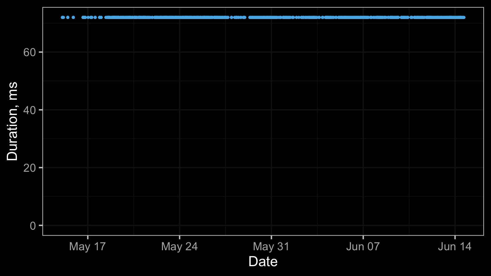
All the observed values are equal, so the corresponding histogram contains a single bin:

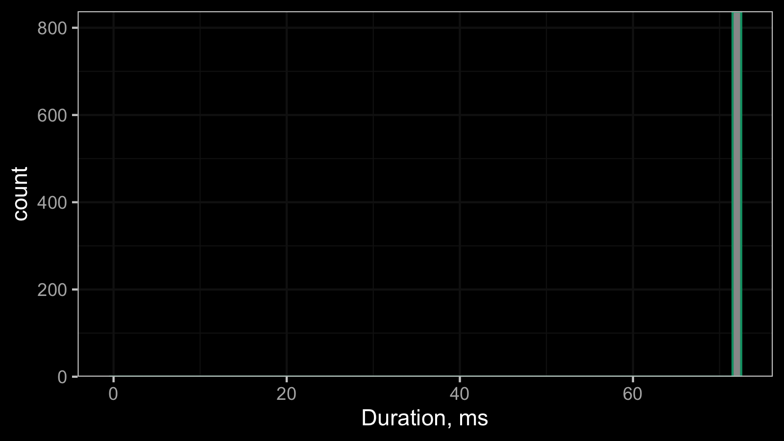
This constant distribution can be described using the Dirac delta function. Non-zero constant distribution is not so typical for time measurements, but it’s a common pattern for advanced performance metrics like the number of garbage collections or the final memory footprint.
Conclusion
The real-life samples are not always easy to analyze. There is always a risk of getting a “corner case” distribution (e.g., with zero dispersion) that will completely break your “general case” equations. If you want to set up an automatic system that works with real-life data, it’s always a good idea to think about such cases in advance and implement corresponding checks.