A better jittering approach for discretization acknowledgment in density estimation

In How to build a smooth density estimation for a discrete sample using jittering, I proposed a jittering approach. It turned out that it does not always work well. It is not always capable of preserving the original distribution shape and avoiding gaps. In this post, I would like to propose a better strategy.

Density estimation is designed to describe continuous distributions. With such a mathematical model, we have an implicit assumption that the probability of observing tied values is zero. Meanwhile, the resolution of the measurement tools is always limited by a finite value, which means that the actually collected observations are essentially discrete. However, when the resolution is much smaller than typical gaps between observations, treating all the distributions as discrete is impractical. The use of continuous models usually provides a decent approximation and more powerful analysis approaches.

When we start reducing the resolution, the discretization effect may appear in the form of occasional tied values. In many real-life applications, this effect is not strong enough to switch to a discrete model, but it prevents us from relying on the “no tied values possible” assumption. Therefore, if we want to build a practically reliable density estimation, we have to handle the tied values properly. Let us review the below examples to better understand the problem.

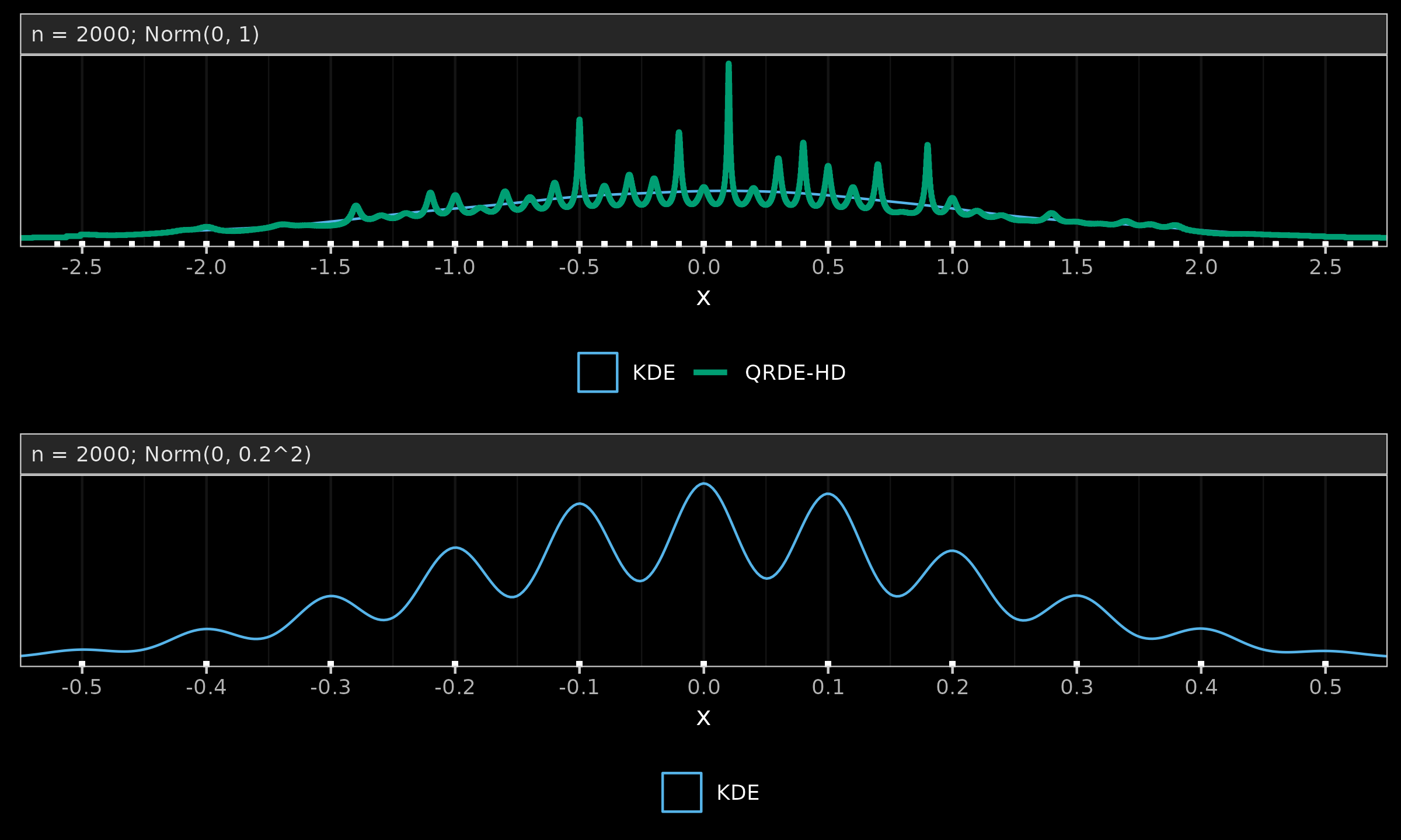
Let us consider a sample of size $2000$ from the standard normal distribution. We round all the measurements to the first decimal digit and build KDE (see The importance of kernel density estimation bandwidth) and QRDE-HD (see Quantile-respectful density estimation based on the Harrell-Davis quantile estimator) which are presented in the below figure (a). While KDE provides a smooth estimation of the normal distribution, QRDE-HD produces spikes at the tied values. The correctness of such a representation is a philosophical question. Indeed, when should we stop considering data as a smooth continuous model and start treating it as a mixture of multiple Dirac delta functions? There is no universal answer: everything depends on the problem and the business needs.

Meanwhile, the discretization effect is relevant not only to QRDE-HD but also to other density estimators. In the below figure (b), we divide the original sample by $5$, round it to the first decimal digit, and build a KDE. As we can see, with a higher number of tied values, KDE also experiences the same phenomenon. The only difference between QRDE-HD and KDE is the tipping point at which the discretization effect becomes noticeable. QRDE-HD has higher sensitivity to ties, which is beneficial for multimodality detection but can be considered a disadvantage in the case of discretization.

While the above examples illustrate an essential limitation of the density estimation approach, they also highlight an important disadvantage of the straightforward QRDE-HD approach. Imagine that we have a sample without tied values and the corresponding QRDE-HD. Next, we decide that the precision of obtained measurements is too high: the last digits of each value are just noise. Therefore, we round the measurements, which leads to tied values. If we are correct and the dropped digits are non-meaningful noise, the rounding procedure does not lead to information loss. Essentially, we still have the same sample. However, the emergence of tied values may prevent us from building reasonably-looking QRDE-HD. That reduces the practical applicability of the suggested approach.

In order to make the density estimation resilient to tied values, we suggest adding noise to the data points in order to spread identical measurements apart. This technique (which is known as jittering, see nagler2018) may feel controversial. While statisticians spend a lot of effort trying to eliminate the noise, jittering suggests distorting the data on purpose. One may have concerns related to the possible efficiency loss or bias introduction. In nagler2018a), a proper justification is provided: it is claimed that jittering does not have a negative impact on the estimation accuracy. According to this work, jittered estimators are not expected to have practically significant deviations from their non-jittered prototypes. While this statement tends to be true in practice, it is worth discussing the details. There are multiple ways to implement jittering. The proper research focus should be on the specific jittering algorithm, not on the concept of jittering in general. In order to choose one, we should define the desired properties first. We suggest the following list of requirements:

• Do not extend the sample range
  The assumption of zero density outside the sample range may be required for further statistical procedure. In order to make jittering applicable for a wider range of use cases, it would be beneficial if we preserve the sample range. For example, if the actual data elements are non-negative by nature and there are tied zero values, a random noise will introduce negative elements, which may be out of the support area for some equations (imagine that a lower percentile value is used inside a square root). Why would we introduce negative elements in such cases if we have an option to change the noise shape and preserve the sample range?
• Use deterministic jittering
  Deterministic behavior is also preferable over non-deterministic if all the other conditions are the same. Any kind of randomization may become a source of flakiness and reduce the reproducibility of analysis. Unlike other statistical methods like bootstrap or Monte-Carlo that intentionally exploit the properties of random distributions, we do not have such a need. The only goal here is to get rid of the tied values. Since the noise is supposed to be negligible, we are free to choose any kind of noise shape. The exact noise pattern can be designed in advance to ensure identical QRDE-HD charts in case of multiple usages of the same data.
• Apply jittering only to the tied values
  Jittering, in general, does not mean that we should add noise to all sample elements. It is reasonable to limit the scope of jittering only to the tied values and avoid unnecessary distortion of unique sample elements.
• The actual resolution from the domain area should be acknowledged
  In order to implement jittering, we should pick up the noise magnitude. We recommend using half of the measure resolution as the maximum deviation from the original value. An approach of estimating the distortion range adaptively based on the observed data is not always applicable. Let us consider a sample of four elements: $\mathbf{x} = (1, 1, 2, 2)$. How should we present it? If we are talking about millimeters and $\mathbf{x}$ was obtained using a ruler with a resolution of 1mm, the noise magnitude of 0.5mm tends to lead to a uniform density or even to a slightly bell-shaped density, which better describes our probable expectations of a high density of around 1.5mm. If we are talking about kilometers and $\mathbf{x}$ contains physical distances measured with a max error of 20 meters, the noise magnitude of 10 meters will lead to a bimodal density with modes at 1km and 2km. Deriving the noise range from the domain area rather than from the sample (e.g., a minimum non-zero distance between sample elements) helps to avoid confusion in corner cases like the one mentioned above.

Such scrutiny may be perceived as unnecessarily elevating minor concerns. However, we believe that it is important to pay due attention to detail. If we can satisfy these requirements for free without any drawbacks and make the implementation applicable to a wider range of corner cases that have a chance to appear in real data sets, we do not observe reasons to avoid this opportunity. We also provide a simple ready-to-use implementation in the end of the post, so that the reader can run it on their data and check if it performs well.

Let us propose a possible noise pattern that satisfies the above requirements. Since we want to prevent noticeable gaps between jittered measurements, it feels reasonable to try the uniform noise. Let $\mathbf{x}_{(i:j)}$ be a range of tied order statistics of width $k=j-i+1$. We want to define a noise vector $\mathbf{x}i_{i:j}$ to obtain the jittered sample $\acute{\mathbf{x}}$ which is defined by

Let $u$ be a vector of indexes $(1,2,\ldots,n)$ linearly mapped to the range $[0;1]$:

We suggest spreading the $\mathbf{x}_{(i:j)}$ values apart using the following rules:

• If ($i > 1$ and $j < n$), we use $\mathbf{x}i_{i:j} = s \cdot (u_{i:j} - 0.5)$.
  In order to support the zero dispersion case, we also use this rule if ($i = 1$ and $j = n$).
• If ($i = 1$ and $j < n$), we use $\mathbf{x}i_{i:j} = s \cdot (u_{i:j} / 2)$.
  Therefore, at the tied values at the minimum value, we extend the range to the right.
• If ($i > 1$ and $j = n$), we use $\mathbf{x}i_{i:j} = s \cdot (u_{i:j} - 1) / 2$.
  Therefore, at the tied values at the maximum value, we extend the range to the left.

The suggested approach preserves the sample range, provides a small bias, and returns consistent non-randomized values. The only case of range extension is a sample of zero-width range, which does not allow for the building of a reasonable density plot preserving equal minimum and maximum values. The knowledge of the resolution value $s$ helps to guarantee the absence of reordering.

The uniform approach works quite well and allows pseudo-restoring of the original noise which is required to protect QRDE-HD from the discretization effect.

Let us consider one more example to show how jittering can restore original density estimation after rounding the sample values.

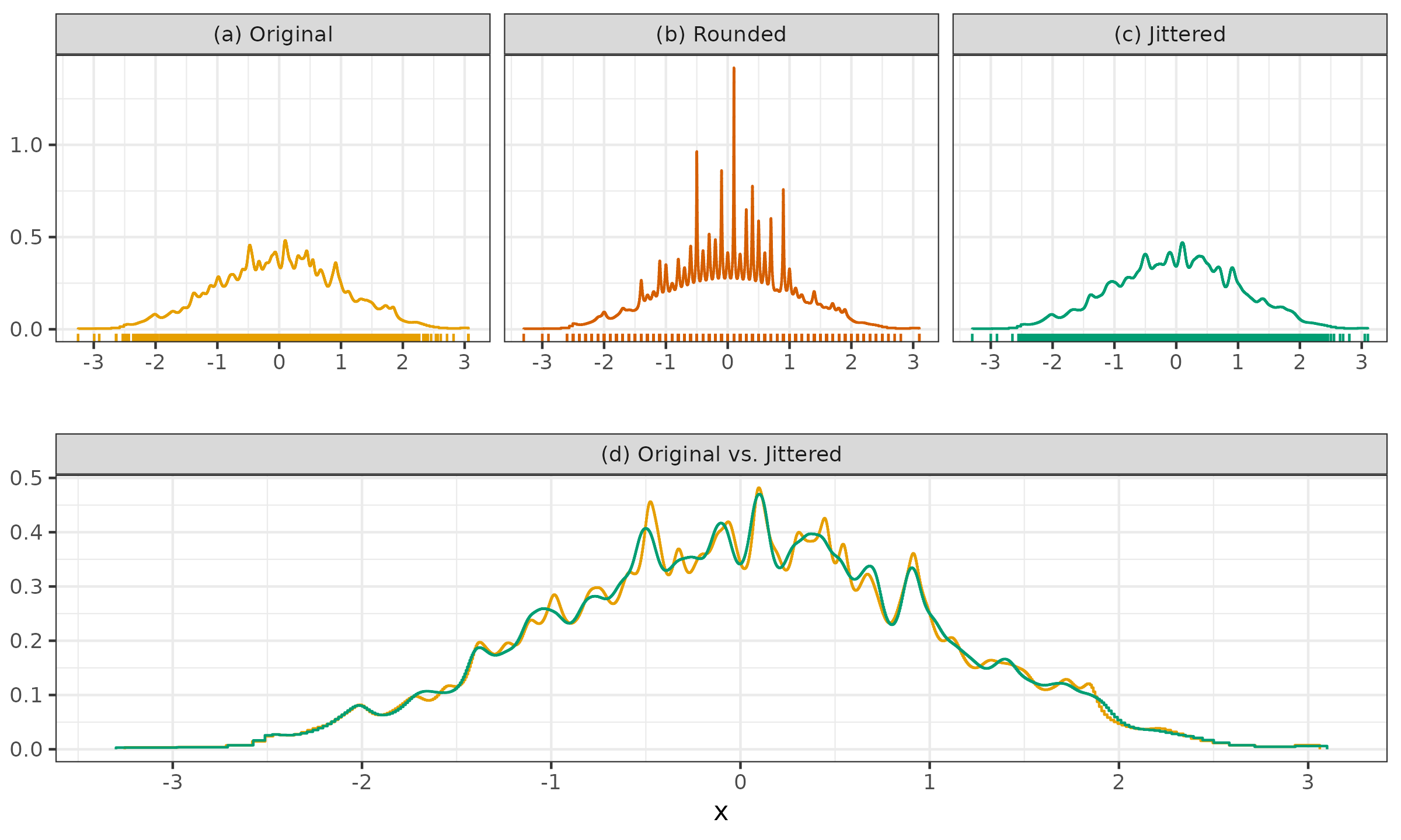
• (a): we can see a QRDE-HD for a sample of 2000 elements from the standard normal distribution.
• (b): we can see a QRDE-HD for a rounded version of the same sample up to the first decimal digit.
• (c): we can see a QRDE-HD for a jittered version of the rounded sample.
• (d): we can see a comparison of the QRDE-HD for the original and jittered sample.

It is easy to see that jittering restored the initial density with minor deviations and helped us overcome the problem of the tied values.

Reference implementation:

#' @param x sample
#' @param s resolution of the measurements
jitter <- function(x, s) {
  x <- sort(x)
  n <- length(x)
  # Searching for intervals [i;j] of tied values
  i <- 1
  while (i <= n) {
    j <- i
    while (j < n && x[j + 1] - x[i] < s / 2) {
      j <- j + 1
    }
    if (i < j && j - i + 1 < n) {
      k <- j - i + 1
      u <- 0:(k - 1) / (k - 1)
      xi <- u - 0.5
      if (i == 1)
        xi <- u / 2
      if (j == n)
        xi <- (u - 1) / 2
      if (i == 1 && j == n)
        xi <- u - 0.5
      x[i:j] <- x[i:j] + xi * s
    
    }
    i <- j + 1
  }
  return(x)
}