Dispersion exponential smoothing

In this previous post, I showed how to apply exponential smoothing to quantiles using the weighted Harrell-Davis quantile estimator. This technique allows getting smooth and stable moving median estimations. In this post, I’m going to discuss how to use the same approach to estimate moving dispersion.

Quantiles

Let’s briefly recall the idea of quantile exponential smoothing. First of all, we should assign exponential weights $w$ to the given timer series $\{ x_1, \ldots, x_n \}$ in the following way:

$$ w_t = e^{-\lambda (n-t)} $$

where $\lambda$ is the decay constant which can be expressed using the half-life value $t_{1/2}$:

$$ \lambda = \frac{\ln(2)}{t_{1/2}}. $$

Next, we should define the weighted Harrell-Davis quantile estimation $q^*_p$ of the $p^\textrm{th}$ quantile:

$$ q^*_p = \sum_{i=1}^{n} W^*_{i} \cdot x_i,\quad W^*_{i} = I_{r^*_i}(a^*, b^*) - I_{l^*_i}(a^*, b^*), $$$$ \left\{ \begin{array}{rcc} l^*_i & = & \dfrac{s_{i-1}(w)}{s_n(w)},\\ r^*_i & = & \dfrac{s_i(w)}{s_n(w)}, \end{array} \right. $$$$ s_i(w) = \sum_{j=1}^i w_j, $$$$ \left\{ \begin{array}{rccl} a^* = & p & \cdot & (n^* + 1),\\ b^* = & (1-p) & \cdot & (n^* + 1), \end{array} \right. $$$$ n^* = \frac{\Big( \sum_{i=1}^n w_i \Big)^2}{\sum_{i=1}^n w_i^2 } $$

where $I_t(a, b)$ is the regularized incomplete beta function.

The same approach can be used with the weighted version of the classic Hyndman-Fan Type 7 quantile estimator (details can be found here).

Dispersion

Once we have a weighted quantile estimator, we can estimate moving measures of dispersion that are based on the quantiles. One of my favorite metrics is the median absolute deviation (MAD):

$$ \textrm{MAD} = \textrm{median}(|x - \textrm{median}(x)|). $$

If we want to use the MAD as the consistency estimator for the standard deviation under normality, we should multiply the above expression by the consistency constant $C_n$:

$$ \textrm{MAD}_n = C_n \cdot \textrm{median}(|x - \textrm{median}(x)|). $$

When the sample is big enough, we can use the asymptotic value as an approximation of $C_n$:

$$ C_\infty = \dfrac{1}{\Phi^{-1}(3/4)} \approx 1.4826022185056 $$

However, for small samples, this constant gives us a biased estimator. In order to get the unbiased estimator, we should properly adjust the value of $C_n$. Note that this value depends on the used quantile estimator. In my previous posts, I already shown how to get proper values for the traditional quantile estimator (here) and the Harrell-Davis quantile estimator (here).

Another way to express the measure of dispersion is the interquartile range (IQR). It’s the difference between upper and lower quartiles:

$$ \textrm{IQR} = Q_3 - Q_1. $$

Since both the MAD and the IQR are based on quantile estimations, we can use calculated them for a given weighted sample.

An example

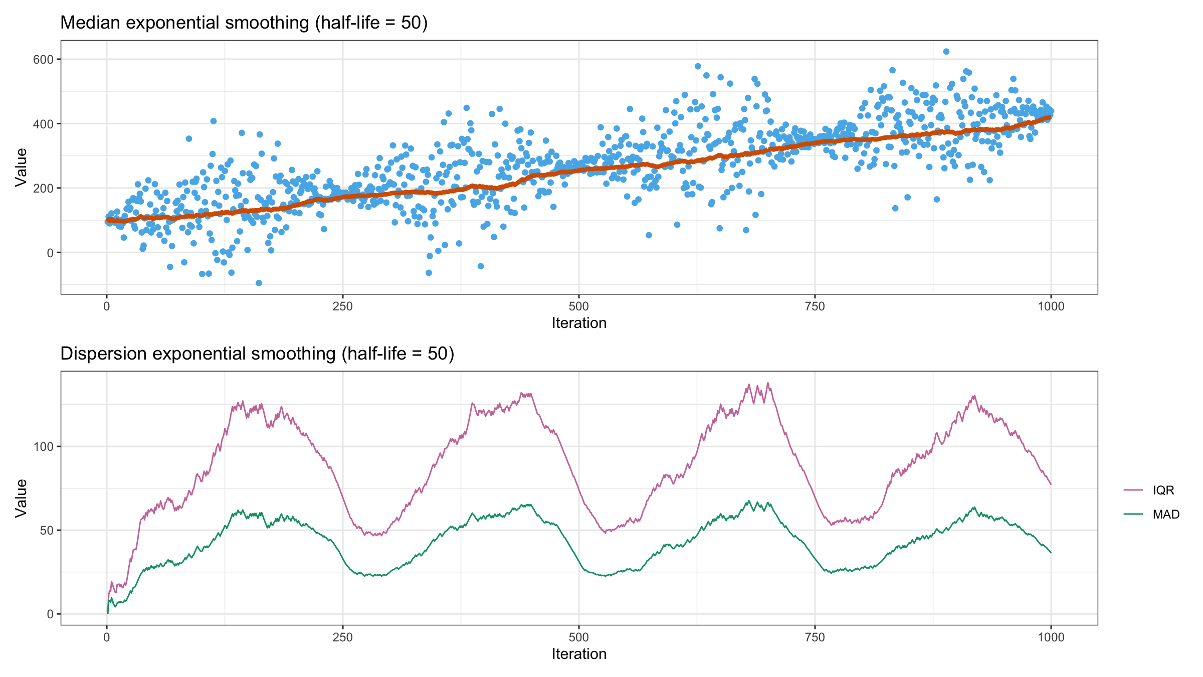
When I test the moving average, I typically use noise sine wave as a primary data pattern. With the moving dispersion, it makes sense to change the data dispersion according to the sine wave. Let’s look at the following figure:

In the upper image, we can observe the raw data point and the estimated moving median using exponential smoothing with half-life = 50. In the bottom picture, we can see the exponentially weighted MAD and IQR. These charts do not only correspond to the actual dispersion, but they also match the previously estimated moving median because they are based on the same weight vector.