Dynamical System Case Study 1 (symmetric 3d system)

Andrey Akinshin · 2022-06-05

Let’s consider the following dynamical system:

{\begin{cases} {\dot{x}}_{1} = f (x_{3}) - x_{1}, \\ {\dot{x}}_{2} = f (x_{1}) - x_{2}, \\ {\dot{x}}_{3} = f (x_{2}) - x_{3}, \end{cases}

where $f (x) = α / (1 + x^{m})$ is a Hill function. In this case study, we explore the phase portrait of this system for $α = 18, m = 3$ .

Preparation

First of all, let’s find the stationary point of this system. Since in such point ${\dot{x}}_{1} = {\dot{x}}_{2} = {\dot{x}}_{3} = 0$ , we have the following equation:

x_{1} = f (f (f ((x_{1})))) .

Since $x_{1}$ is monotonically increasing and $f (f (f (x_{1}))))$ is monotonically decreasing, this equation has exactly one solution. It’s easy to see that this solution is $x_{0} = x_{1} = x_{2} = x_{3} = 2$ .

Next, we build the corresponding linearization matrix:

M = [\begin{matrix} - 1 & 0 & f^{'} (x_{0}) \\ f^{'} (x_{0}) & - 1 & 0 \\ 0 & f^{'} (x_{0}) & - 1 \end{matrix}] .

Since $f^{'} (x) = - α m x^{m - 1} / (x^{m} + 1)^{2}$ , we have:

f^{'} (x_{0}) = - 18 * 3 * 2^{2} / (2^{3} + 1)^{2} = - 216 / 81 = - 8 / 3 \approx - 2.66667 .

Thus,

M = [\begin{matrix} - 1 & 0 & - 8 / 3 \\ - 8 / 3 & - 1 & 0 \\ 0 & 8 / 3 & - 1 \end{matrix}] .

Now we can get the eigenvalues $λ_{i}$ and eigenvectors $e_{i}$ :

λ_{1} \approx - 3.666667, λ_{2} \approx 0.333333 + 2.309401 i, λ_{3} \approx 0.333333 - 2.309401 i,

[\begin{matrix} e_{1} \\ e_{2} \\ e_{3} \end{matrix}] = [\begin{matrix} - 0.5773503, & - 0.5773503, & - 0.5773503 \\ - 0.2886751 + 0.5 i, & - 0.2886751 - 0.5 i, & 0.5773503 \\ - 0.2886751 - 0.5 i, & - 0.2886751 + 0.5 i, & 0.5773503 \end{matrix}] .

The most expressive phase portrait could be obtained using a projection on $(e_{2}, e_{3})$ or $(ℜ (e_{2}), ℑ (e_{2})) = (ℜ (e_{3}), - ℑ (e_{3}))$ .

Phase portraits

In order to explore phase portraits, we perform several simulation studies. In each simulation, we generate several trajectories from random start points and draw three plots:

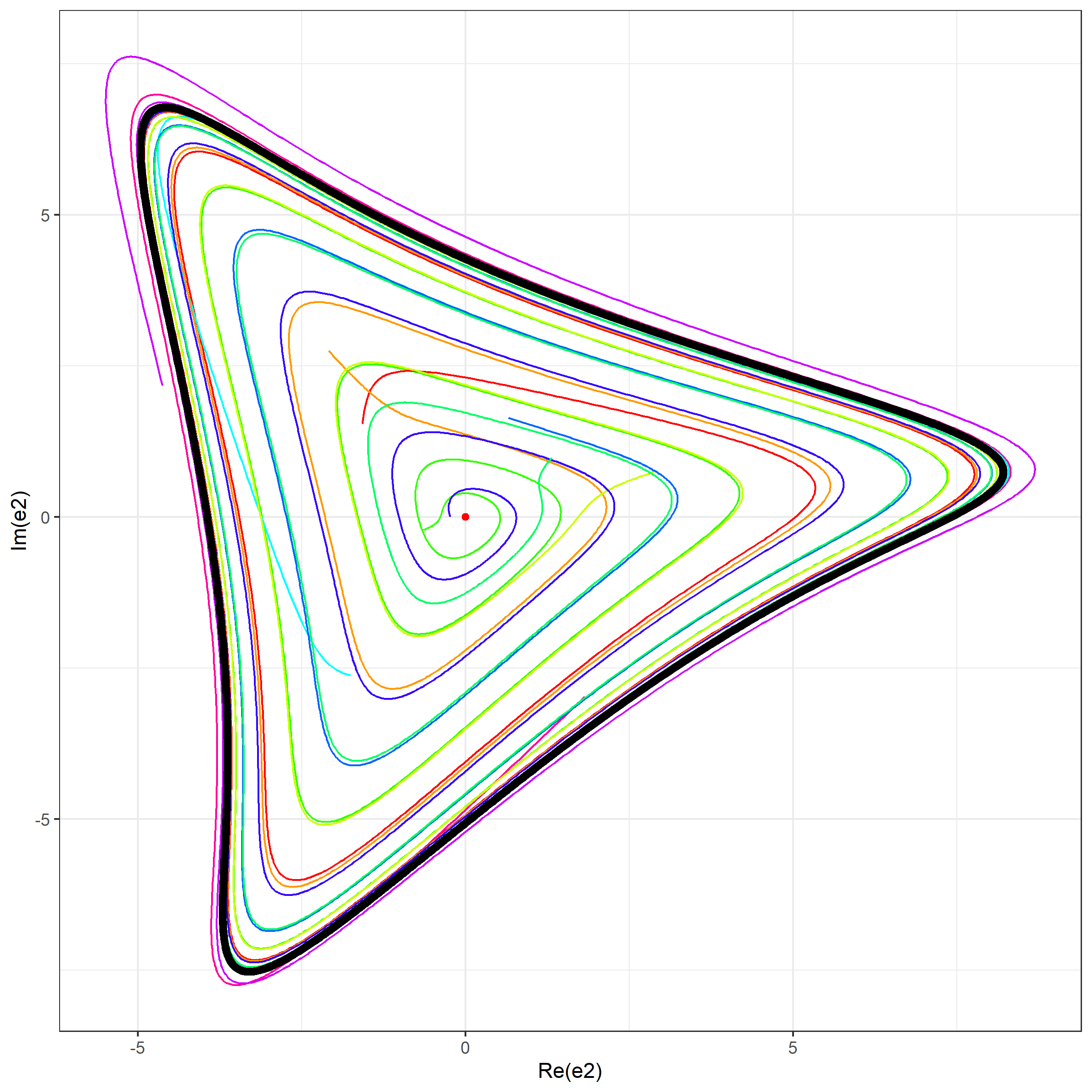
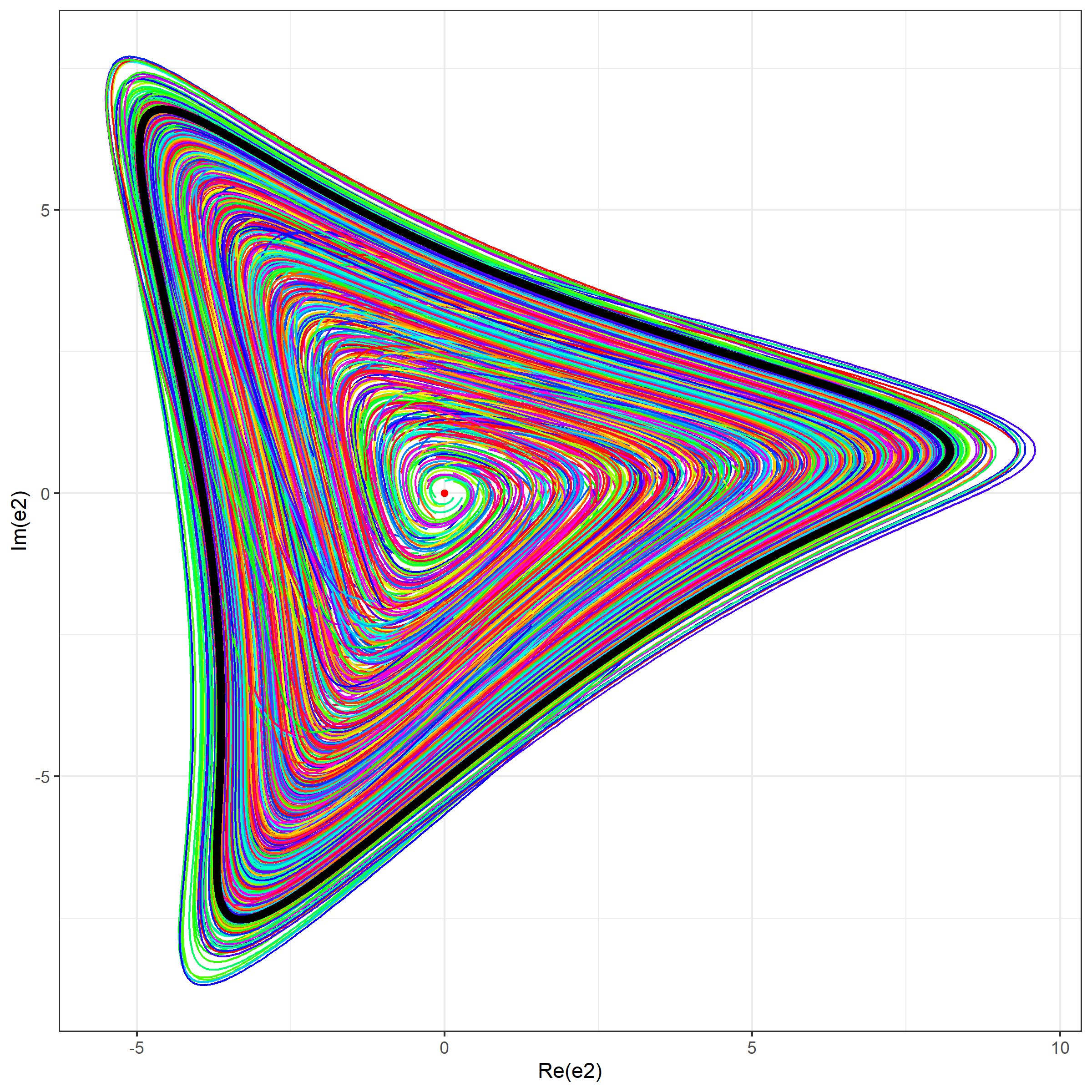
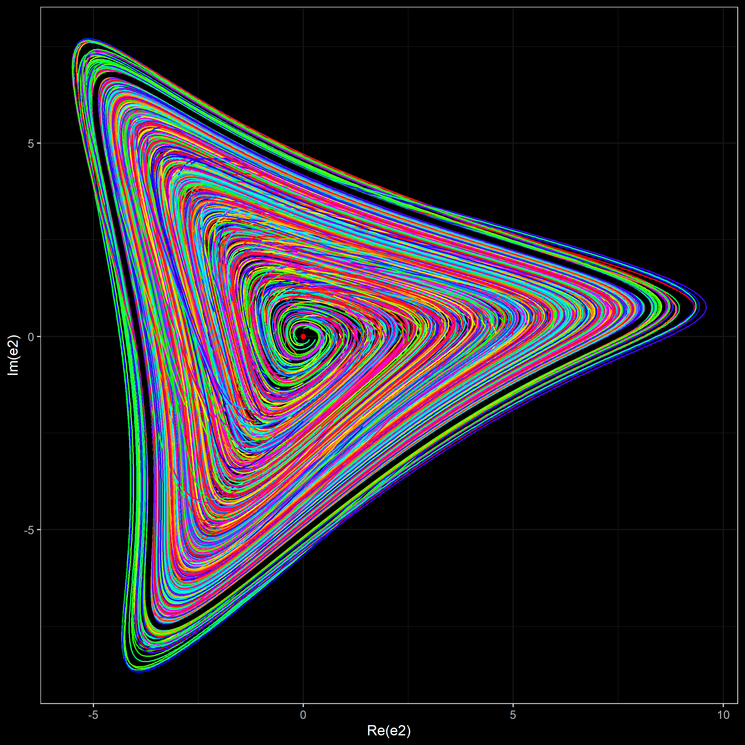
A projection of simulated trajectories on $(ℜ (e_{2}), ℑ (e_{2}))$ . Each trajectory has own color from a rainbow palette. The limit cycle is shown using the black color.
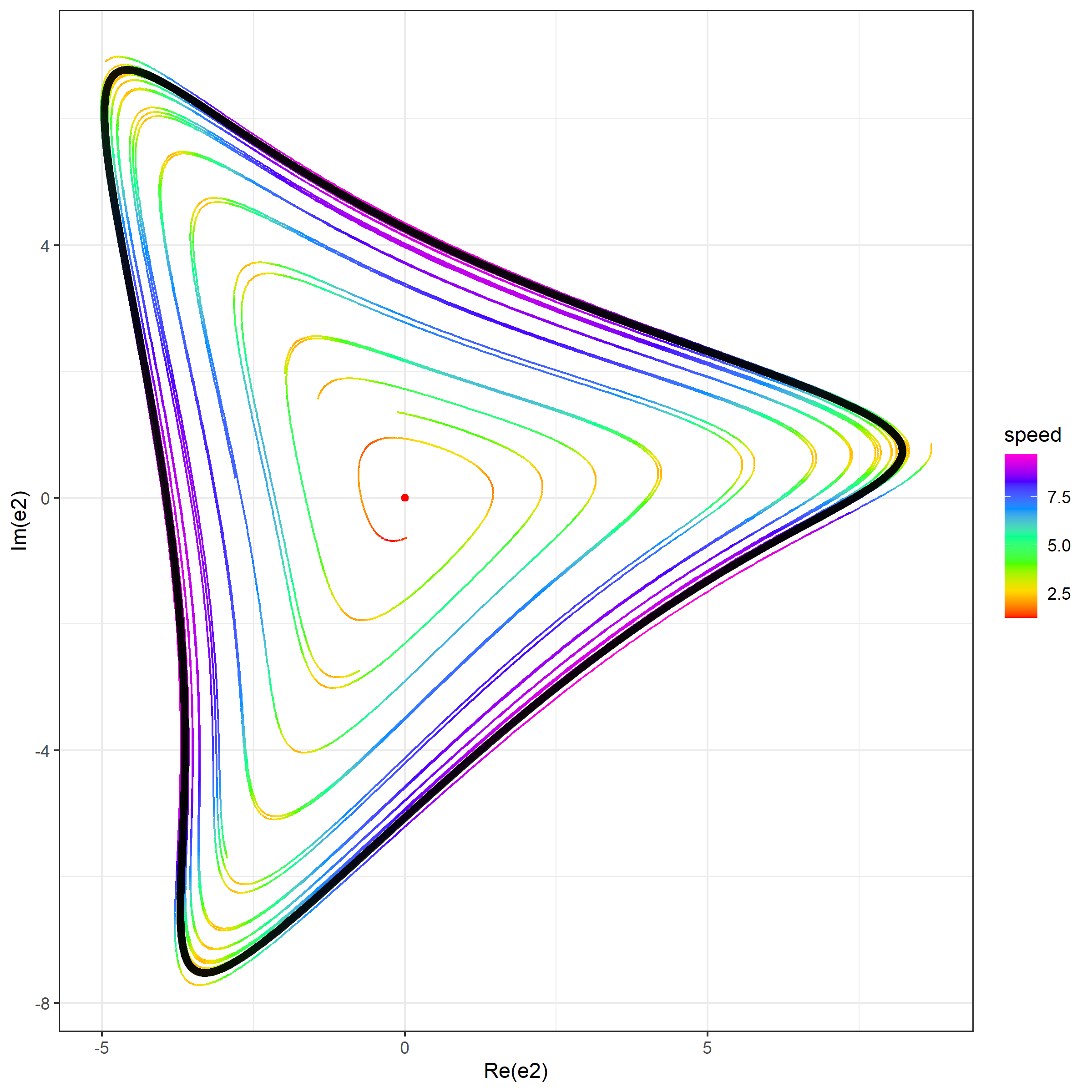
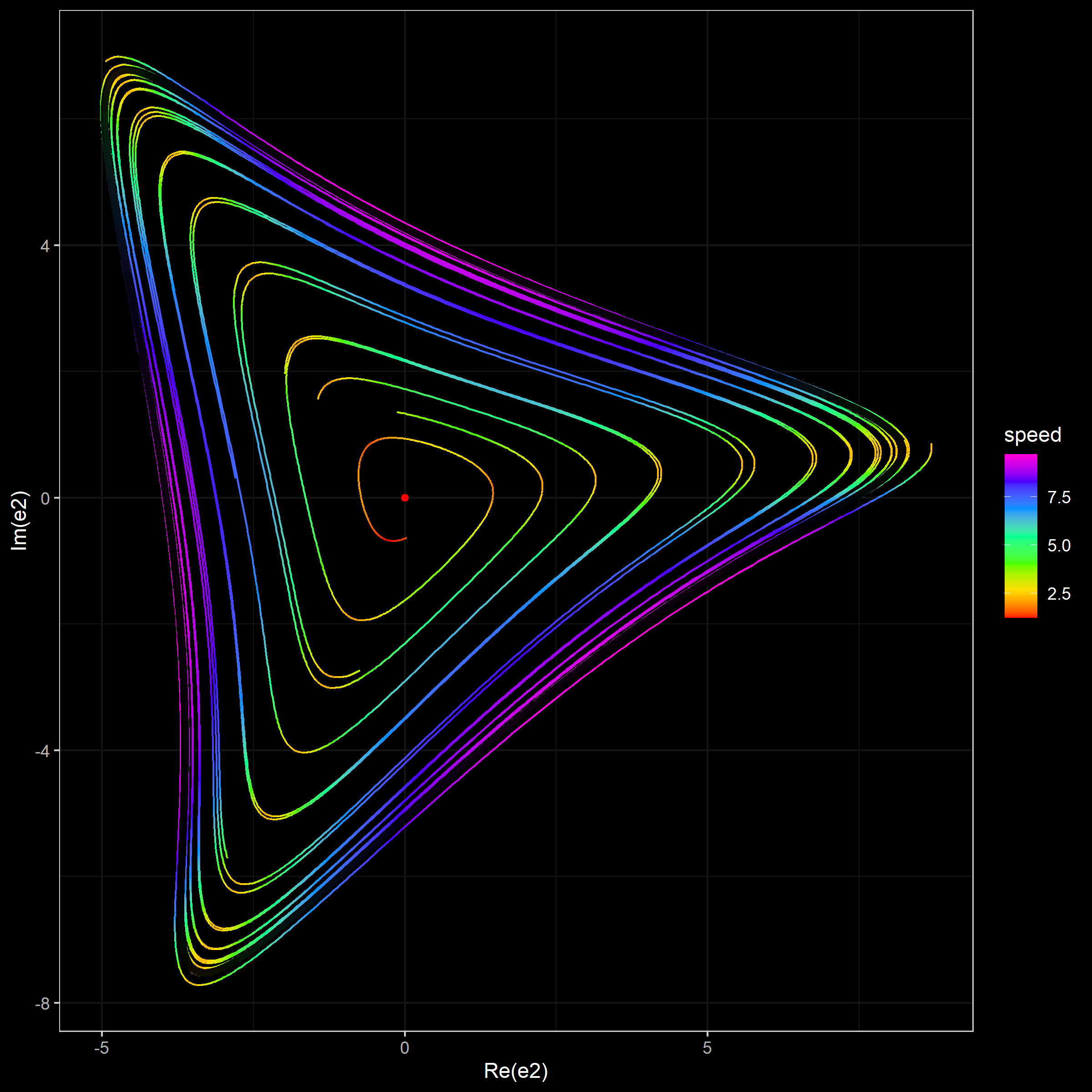
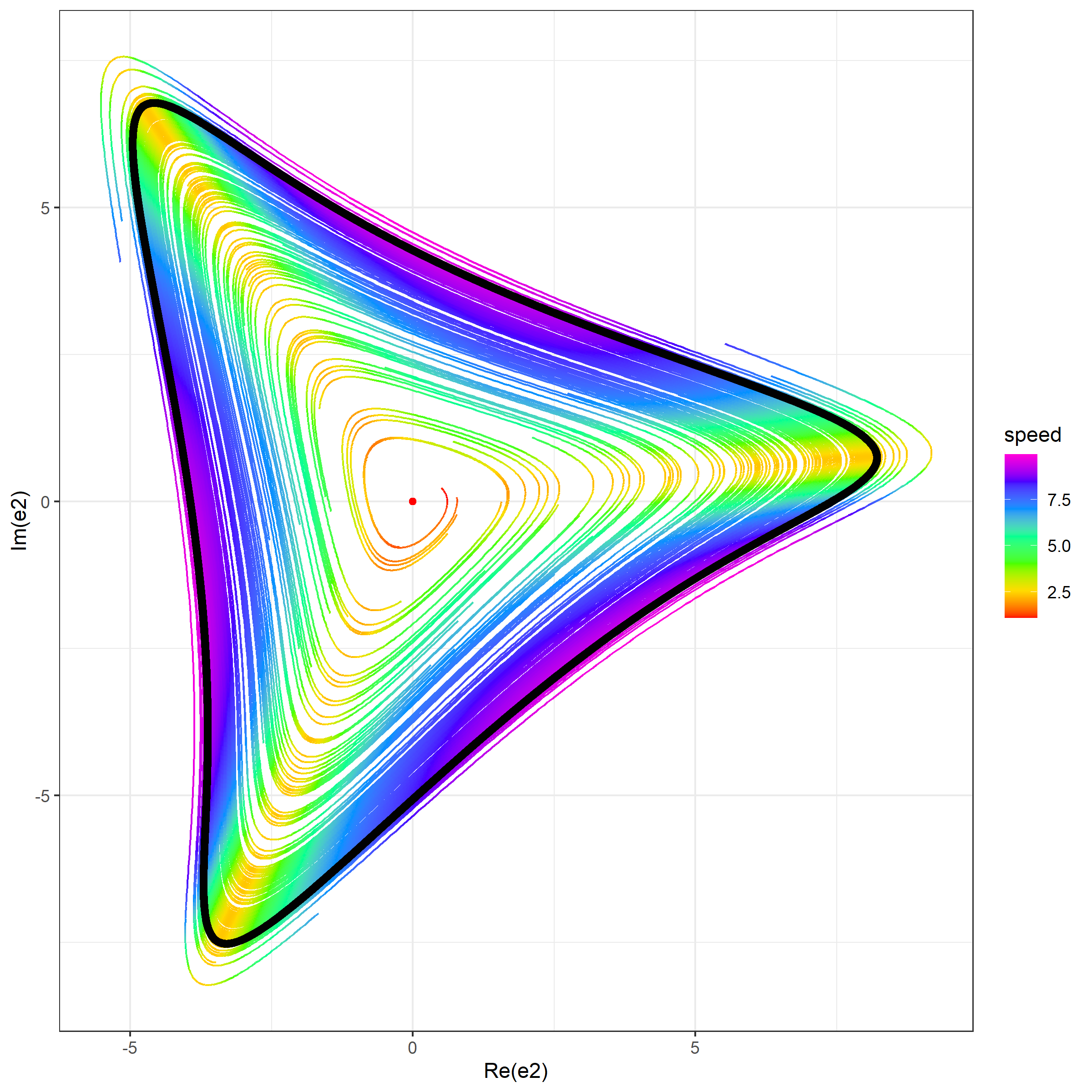
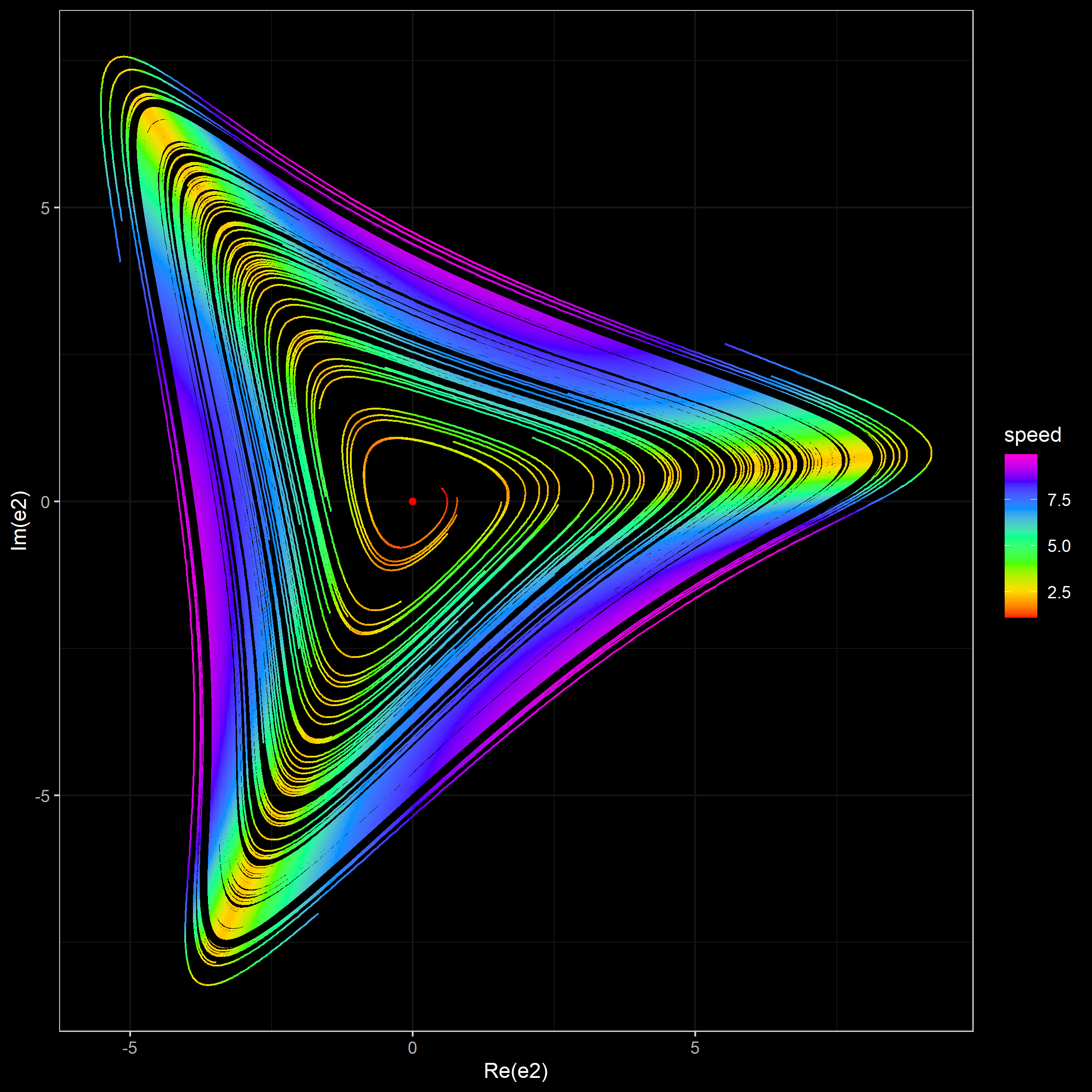
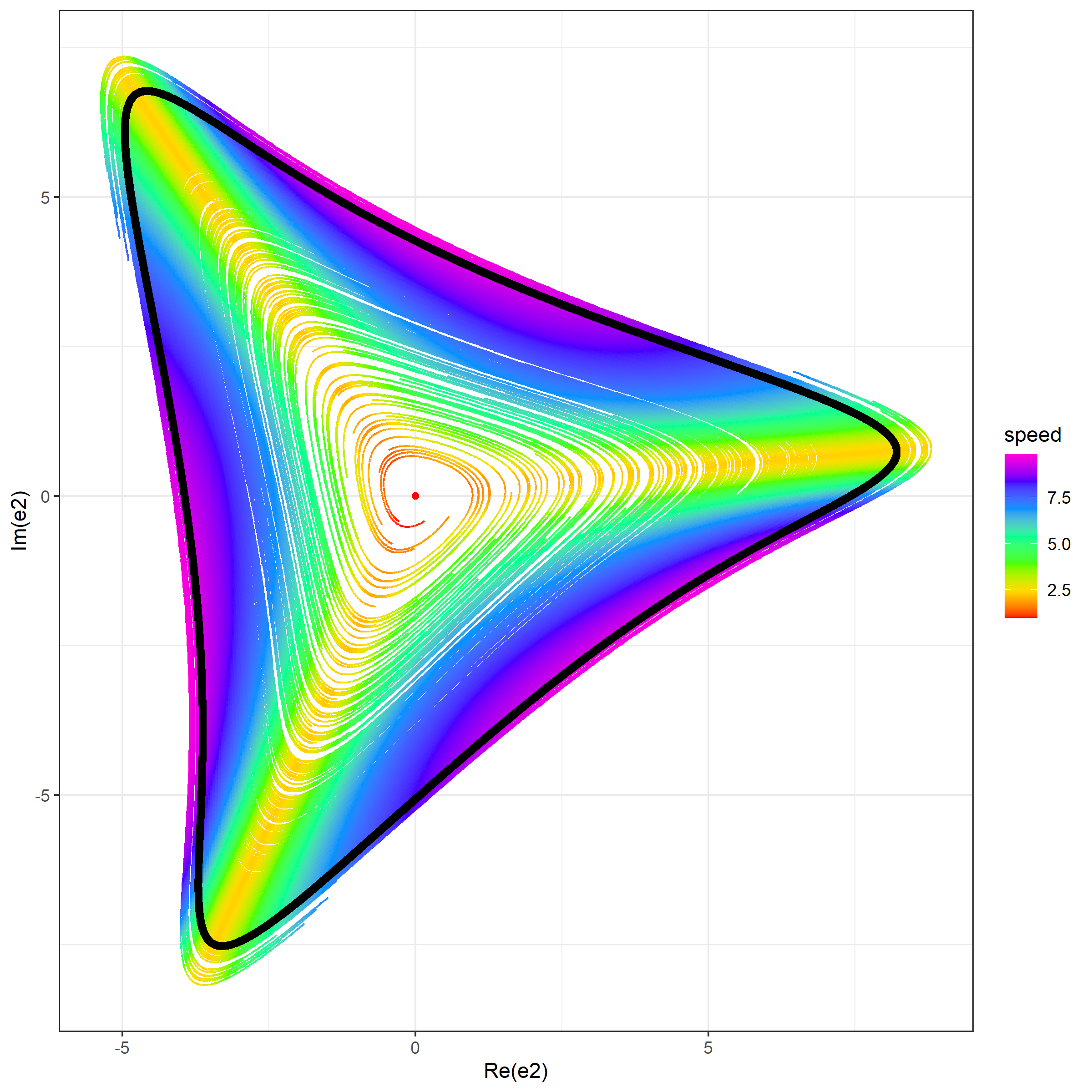
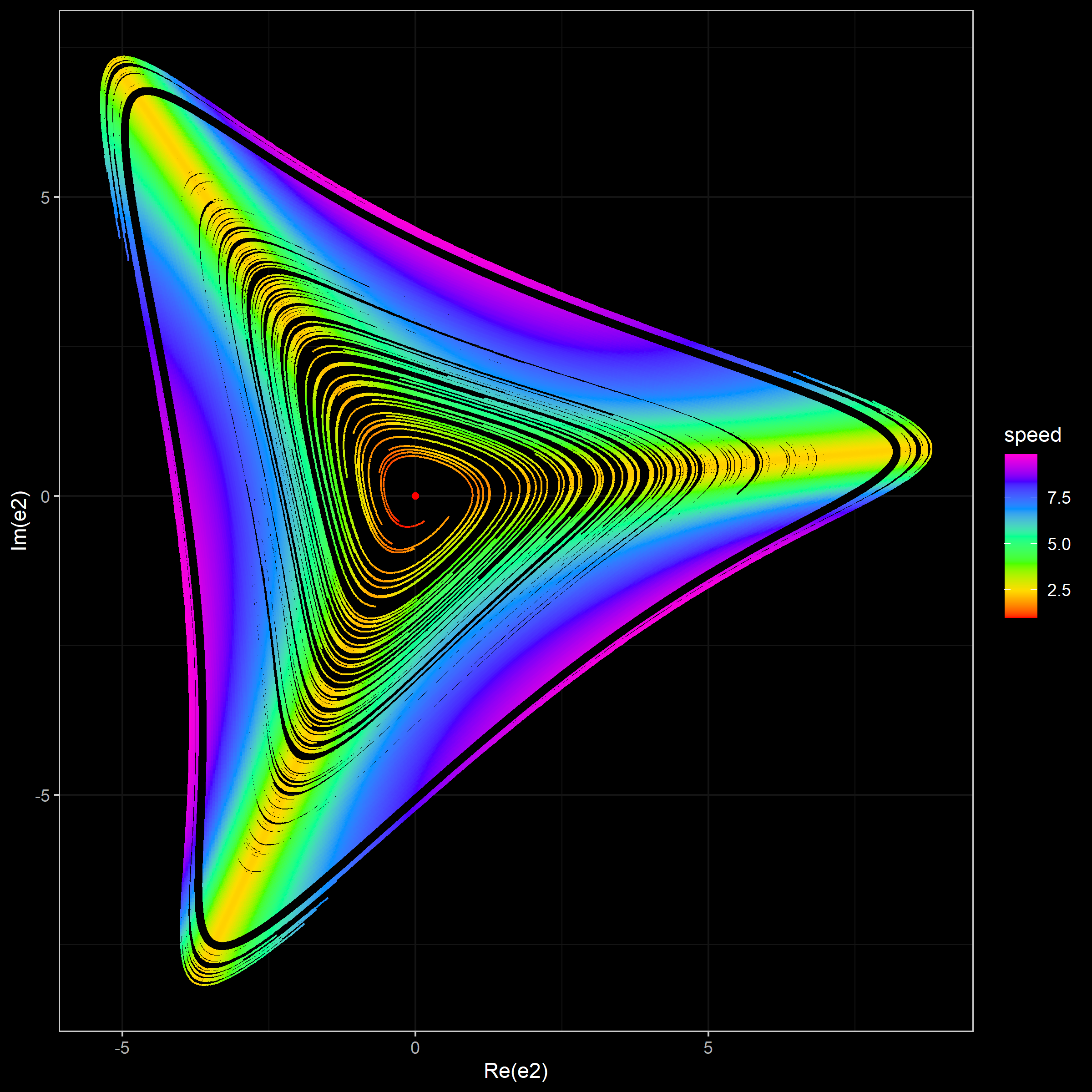
A projection of simulated trajectories on $(ℜ (e_{2}), ℑ (e_{2}))$ . For each trajectory point, the color defines the current speed ( $\sqrt{{\dot{x}}_{1}^{2} + {\dot{x}}_{2}^{2} + {\dot{x}}_{3}^{2}}$ ). The limit cycle is shown using the black color. The beginning of each trajectory is drop in order to provide a more consistent picture.
A 3D projection of simulation trajectories on $(e 1_{,} ℜ (e_{2}), ℑ (e_{2}))$ . These visualizations are heavy, so you should click on “Show 3D plot” in order to explore the plot.

Simulation 1 (10 trajectories)

In this simulation, we generate 10 trajectories from random start points around the stationary point uniformly taken in $(x_{1}, x_{2}, x_{3})$ .

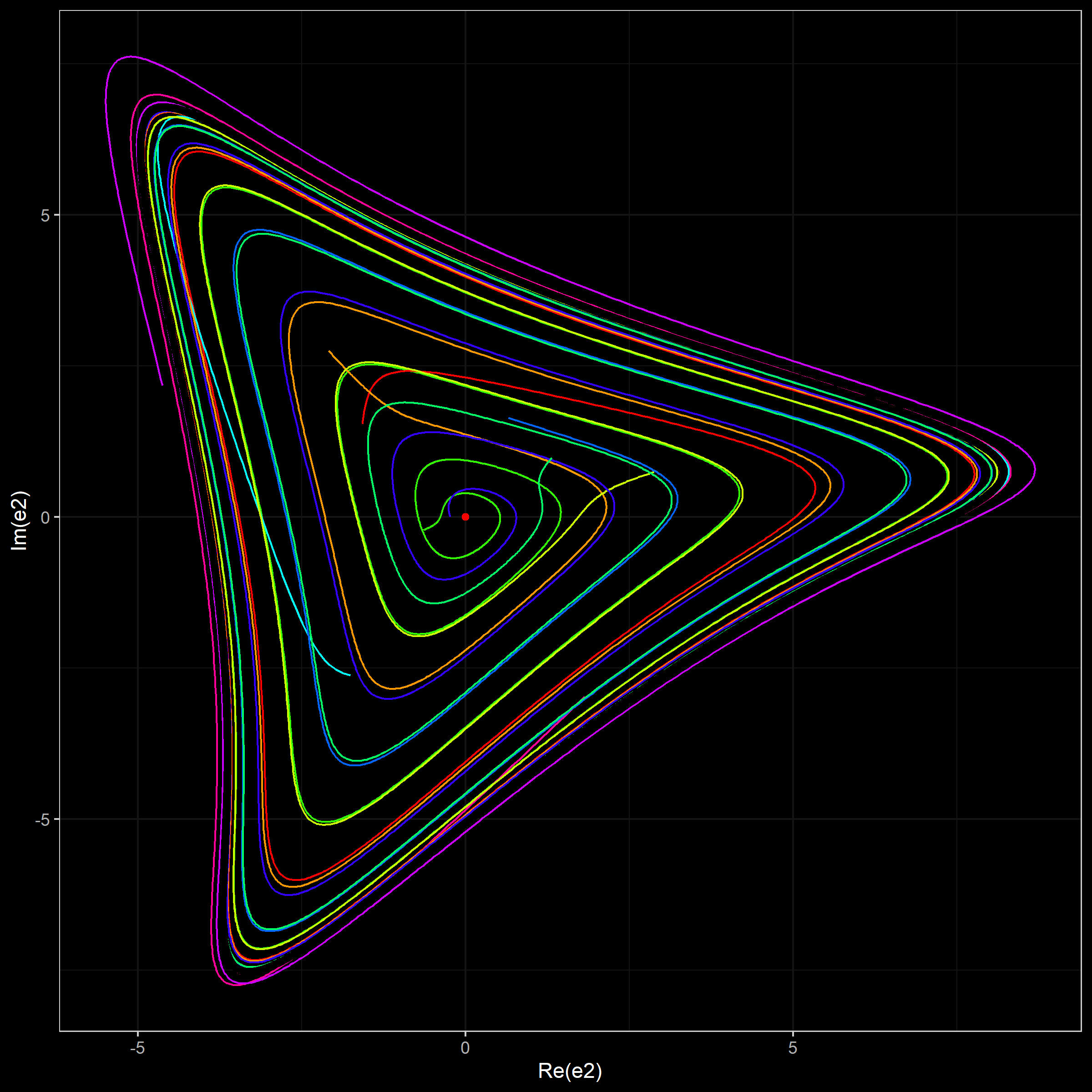
Simulation 2 (100 trajectories)

In this simulation, we generate 100 trajectories from random start points around the stationary point uniformly taken in $(x_{1}, x_{2}, x_{3})$ .

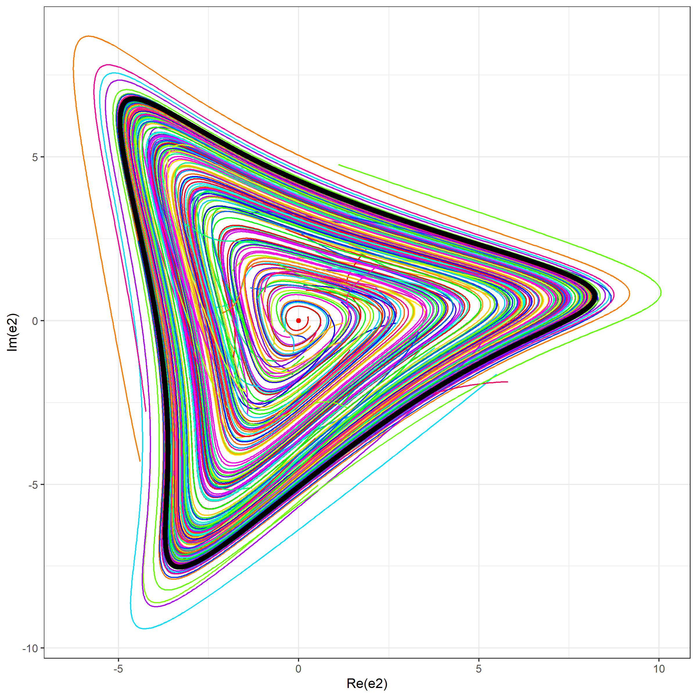
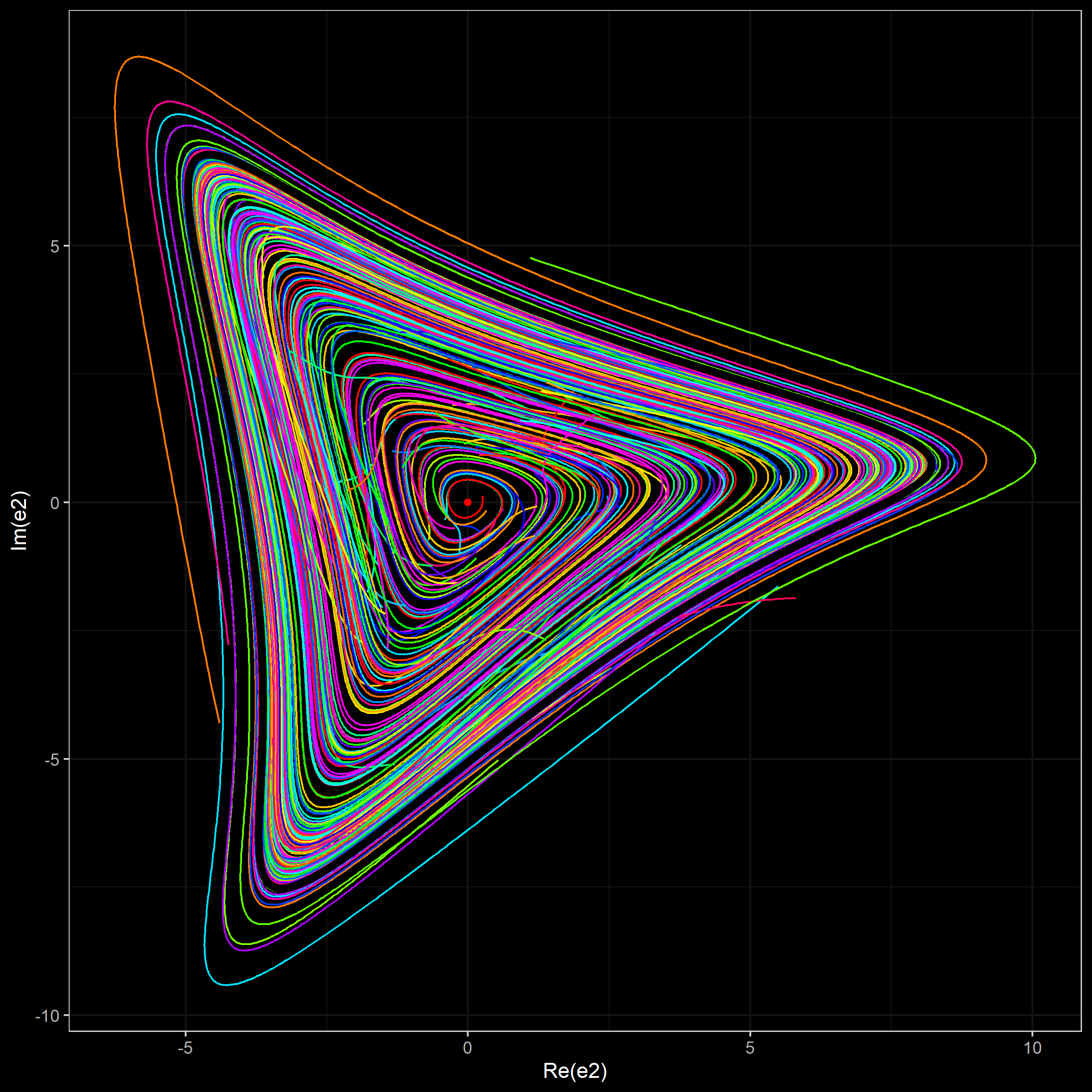
Simulation 3 (500 trajectories)

In this simulation, we generate 500 trajectories from random start points around the stationary point uniformly taken in $(e_{1}, e_{2}, e_{3})$ .

Source code

library(deSolve)
library(ggplot2)
library(dplyr)
library(tidyr)
library(plotly)

simParams <- list(
  totalTime = 50,
  step = 0.01,
  startThreshold = 3,
  endThreshold = 45
)

hypot <- function(x, y) sqrt(x^2 + y^2)
fp <- list(a = 18, m = 3)
f <- function(x, a = fp$a, m = fp$m) a / (1 + x ^ m)
df <- function(x, a = fp$a, m = fp$m) -a * m * x ^ (m - 1) / (x ^ m + 1)^2

model <- function(t, x, parms) {
  with(as.list(c(parms, x)), {
    dx1 <- f(x3) - x1
    dx2 <- f(x1) - x2
    dx3 <- f(x2) - x3
    list(c(dx1, dx2, dx3))
  })
}
calc.speed <- function(x) sqrt(sum(unlist(model(0, x, 0))^2))

x0 <- uniroot(function(x) f(f(f(x)))-x, c(0, fp$a), tol = 1e-9)$root
M <- matrix(c(
  -1, 0, df(x0),
  df(x0), -1, 0,
  0, df(x0), -1
), nrow = 3, ncol = 3, byrow = TRUE)
eigenM <- tryCatch(eigen(M), error = function(e) list(values = rep(NA, 6), vectors = matrix(rep(NA, 36), ncol = 6)))
Ml <- eigenM$values
Me <- eigenM$vectors

simulate <- function(name, start) {
  times  <- seq(0, simParams$totalTime, by = simParams$step)
  traj <- data.frame(lsoda(start, times, model, c()))
  traj$speed <- sapply(1:nrow(traj), function(index) calc.speed(traj[index, 2:4]))

  proj <- function(e){
    dotProduct <- rowSums(t(t((traj[,2:4]) - x0) * e))
    l <- sqrt(sum(e^2))
    dotProduct / l
  }
  traj$e1 <- proj(Re(Me[,1]))
  traj$e2 <- proj(Re(Me[,2]))
  traj$e3 <- proj(Im(Me[,2]))
  traj$name <- name
  traj
}
generate.input <- function(type, maxTraj = -1) {
  if (type == 1) {
    if (maxTraj <= 0)
      maxTraj <- 1
    return(data.frame(
      x1 = abs(x0 + rnorm(maxTraj) * 3),
      x2 = abs(x0 + rnorm(maxTraj) * 3),
      x3 = abs(x0 + rnorm(maxTraj) * 3)
    ))
  }
  if (type == 2) {
    input <- expand.grid(e2 = seq(-5, 8, by = 0.2), e3 = seq(-7.5, 7, by = 0.2))
    noise <- runif(nrow(input), -5, 5)
    ue1 <- Re(Me[,1])
    ue2 <- Re(Me[,2])
    ue3 <- Im(Me[,2])
    input$x1 <- noise * ue1[1] + input$e2 * ue2[1] + input$e3 * ue3[1]
    input$x2 <- noise * ue1[2] + input$e2 * ue2[2] + input$e3 * ue3[2]
    input$x3 <- noise * ue1[3] + input$e2 * ue2[3] + input$e3 * ue3[3]
    input <- input[input$x1 > 0 & input$x2 > 0 & input$x3 > 0,]
    if (maxTraj > 0 & maxTraj < nrow(input))
      input <- input[sample(1:nrow(input), maxTraj),]
    return(input)
  }
  stop("Unknown type")
}
simulate2 <- function(input) {
  get.input <- function(i) c(x1 = input[i, "x1"], x2 = input[i, "x2"], x3 = input[i, "x3"])
  do.call("rbind", lapply(1:nrow(input), function(i) simulate(paste0("t", i), get.input(i))))
}

draw.simple <- function(traj) {
  ggplot(traj, aes(e2, e3, col = name)) +
    geom_path(aes(group = name)) +
    geom_point(aes(x, y), data.frame(x = 0, y = 0), col = "red") +
    geom_path(aes(e2, e3, group = name), traj[traj$time > simParams$endThreshold,], col = "black", size = 2, alpha = 0.1) +
    scale_color_manual(values = sample(rainbow(length(unique(traj$name))))) +
    theme(legend.position="none") +
    labs(x = "Re(e2)", y = "Im(e2)")
}
draw.speed <- function(traj) {
  ggplot(traj[traj$time > simParams$startThreshold,], aes(e2, e3, col = speed)) +
    geom_path(aes(group = name)) +
    geom_point(aes(x, y), data.frame(x = 0, y = 0), col = "red") +
    geom_path(aes(e2, e3, group = name), traj[traj$time > simParams$endThreshold,], col = "black", size = 2, alpha = 0.1) +
    scale_color_gradientn(colours = rainbow(7)) +
    labs(x = "Re(e2)", y = "Im(e2)")
}
draw.3d <- function(traj) {
  traj3d <- traj[traj$time > simParams$startThreshold,c("time", "e1", "e2", "e3", "name")]
  traj3d[,2:4] <- round(traj3d[,2:4], 3) # Compressing
  plot_ly(
    traj3d, x = ~e1, y = ~e2, z = ~e3,
    type = 'scatter3d', mode = 'lines', opacity = 1, color = ~name,
    colors = sample(rainbow(length(unique(traj$name))))) %>%
    layout(showlegend = FALSE)
}


# Simulation 1
set.seed(1)
traj1 <- simulate2(generate.input(1, 10))
# draw.simple(traj1)
# draw.speed(traj1)
# draw.3d(traj1)

# Simulation 2
set.seed(2)
traj2 <- simulate2(generate.input(1, 100))
# draw.simple(traj2)
# draw.speed(traj2)
# draw.3d(traj2)

# Simulation 3
set.seed(3)
traj3 <- simulate2(generate.input(2))
# draw.simple(traj3)
# draw.speed(traj3)
# draw.3d(traj3)