Folded medians
In the previous post, we discussed the Gastwirth’s location estimator. In this post, we continue playing with different location estimators. To be more specific, we consider an approach called folded medians. Let $x = \{ x_1, x_2, \ldots, x_n \}$ be a random sample with order statistics $\{ x_{(1)}, x_{(2)}, \ldots, x_{(n)} \}$. We build a folded sample using the following form:
$$ \Bigg\{ \frac{x_{(1)}+x_{(n)}}{2}, \frac{x_{(2)}+x_{(n-1)}}{2}, \ldots, \Bigg\}. $$If $n$ is odd, the middle sample element is folded with itself. The folding operation could be applied several times. Once folding is conducted, the median of the final folded sample is the folded median. A single folding operation gives us the Bickel-Hodges estimator.
In this post, we briefly check how this metric behaves in the case of the Normal and Cauchy distributions.
Simulation study
Let’s conduct the following simulation:
- Enumerate different samples sizes $n = \{ 10, 20, 50 \}$
- Enumerate different location estimators: Gastwirth’s location estimator $Q_{\operatorname{G}}$, the sample median $Q_{\operatorname{SM}}$, the Harrell-Davis median estimator $Q_{\operatorname{HD}}$, the Hodges-Lehmann median estimator $Q_{\operatorname{HL}}$, and three folded medians $Q_{\operatorname{FM1}}$, $Q_{\operatorname{FM2}}$, $Q_{\operatorname{FM3}}$ with one, two, and three foldings respectively.
- Enumerate different distributions: the standard Normal distribution, the standard Cauchy distribution
- For each sample size, estimator, and distribution, generate $10\,000$ random samples of the given size from the given distribution and calculate the location estimation using the given estimator.
- Draw the corresponding density plots for the obtained estimation using Sheather & Jones method and the normal kernel.
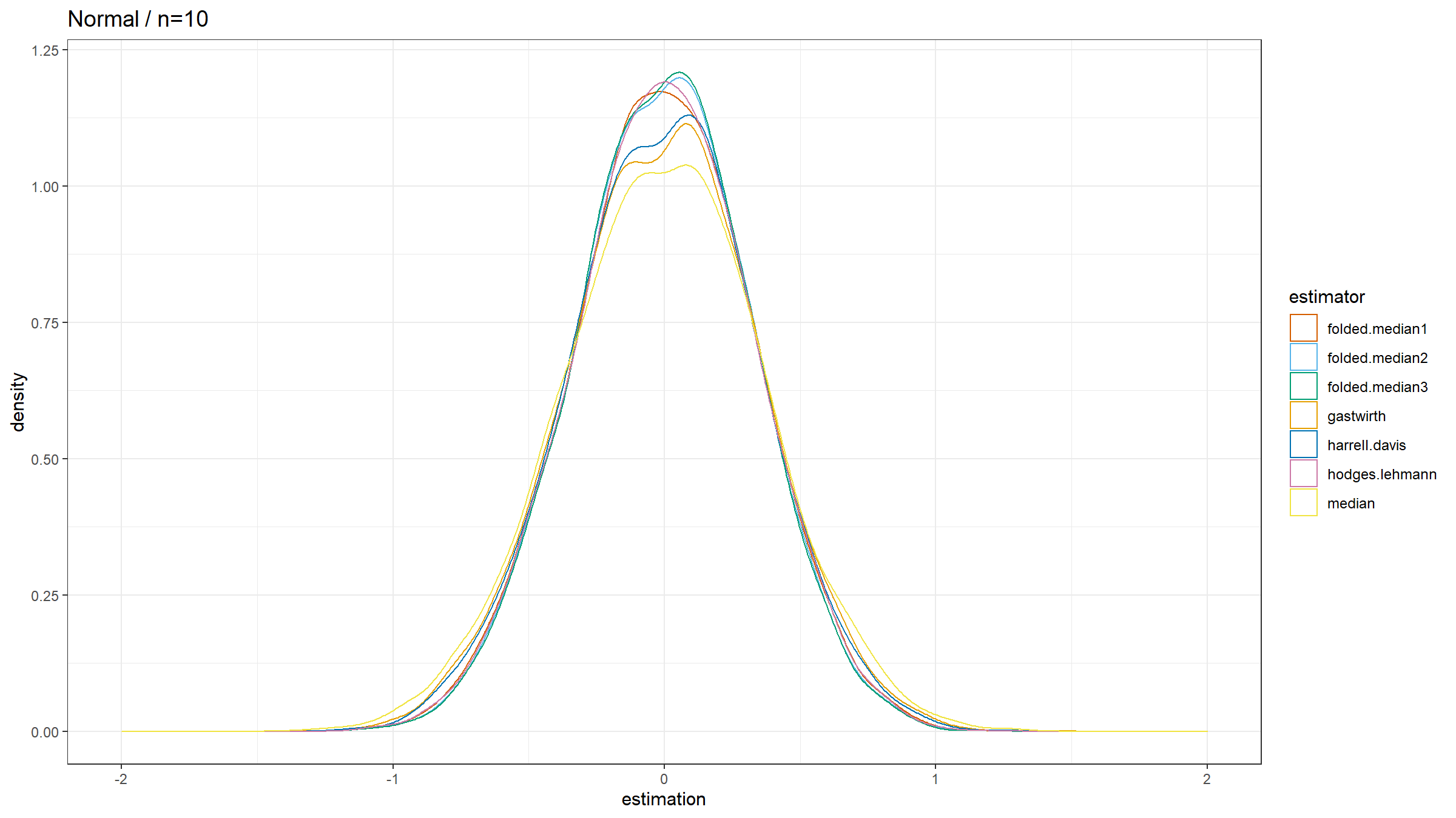
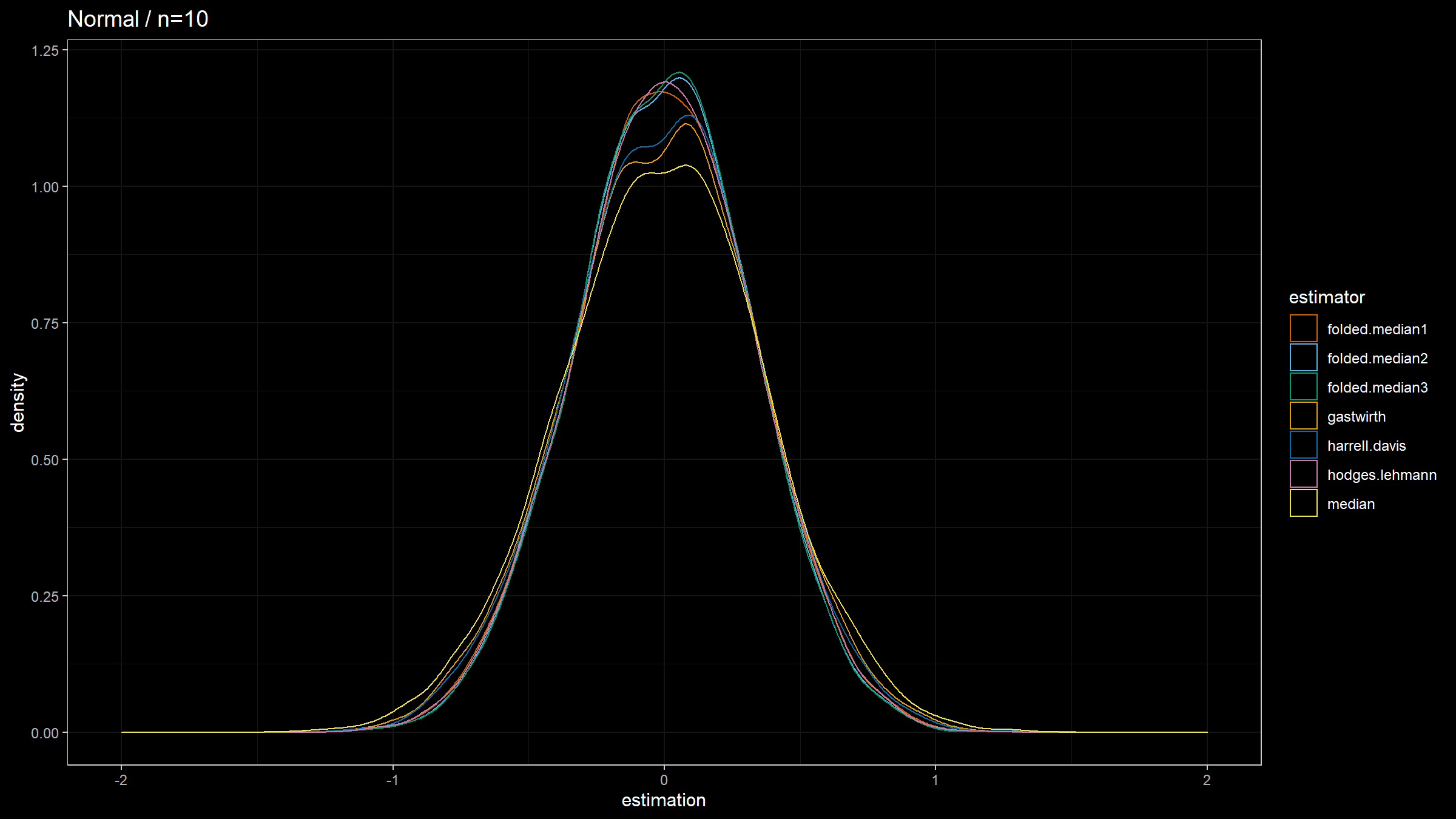
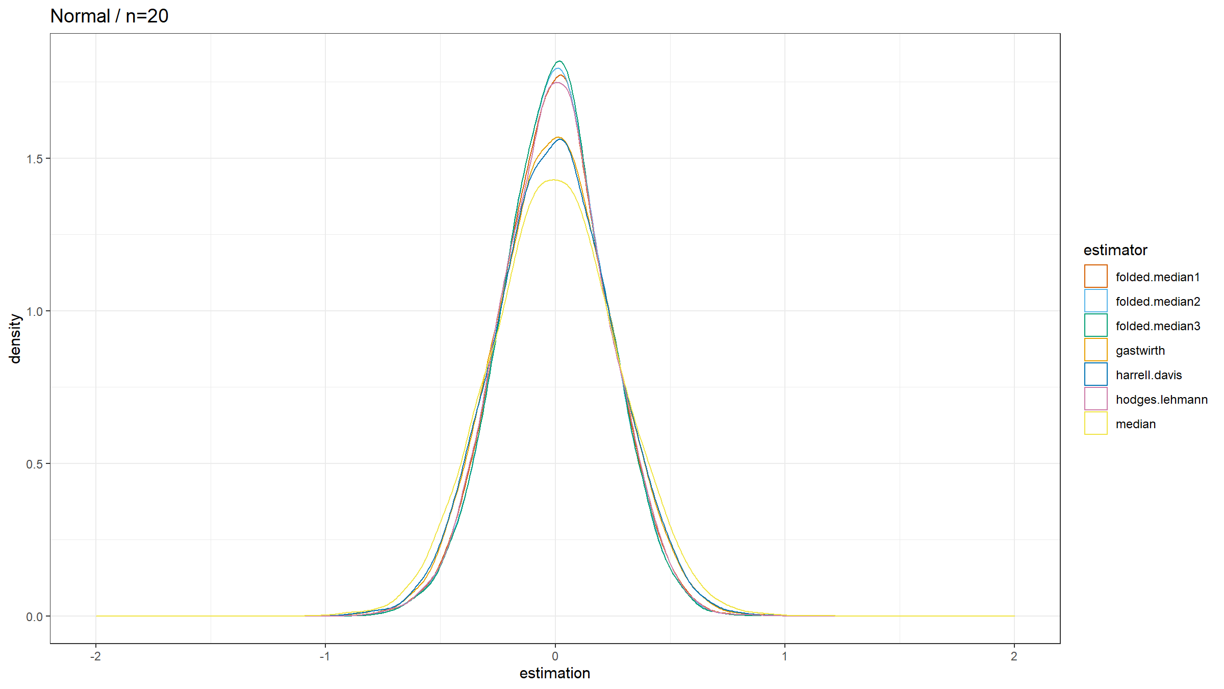
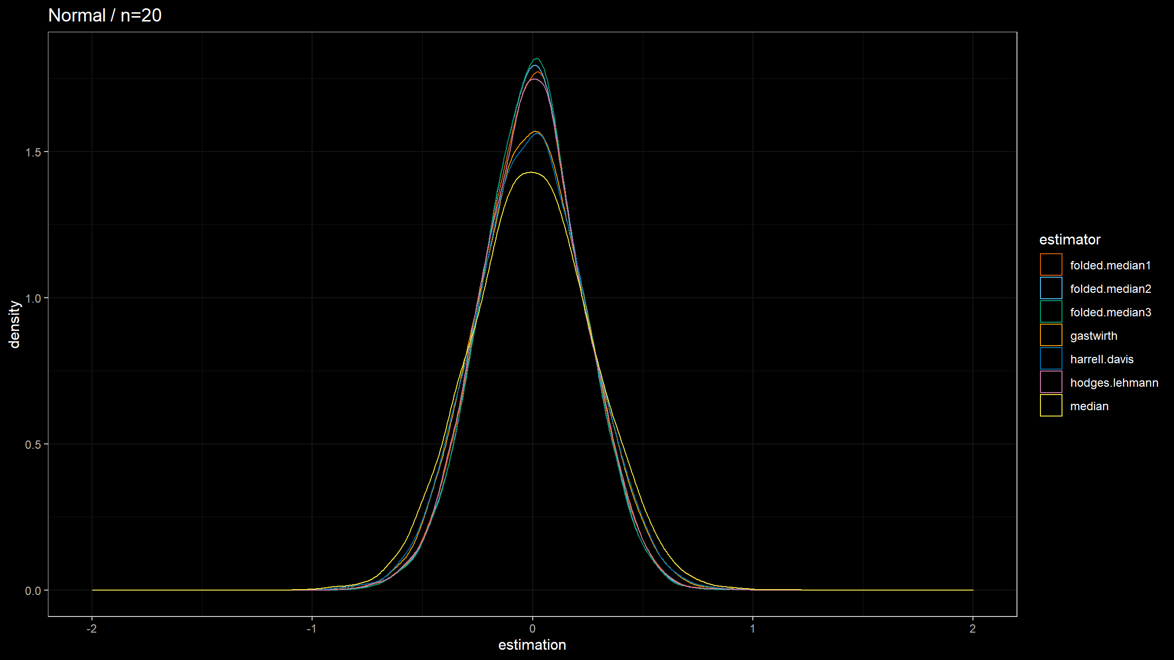
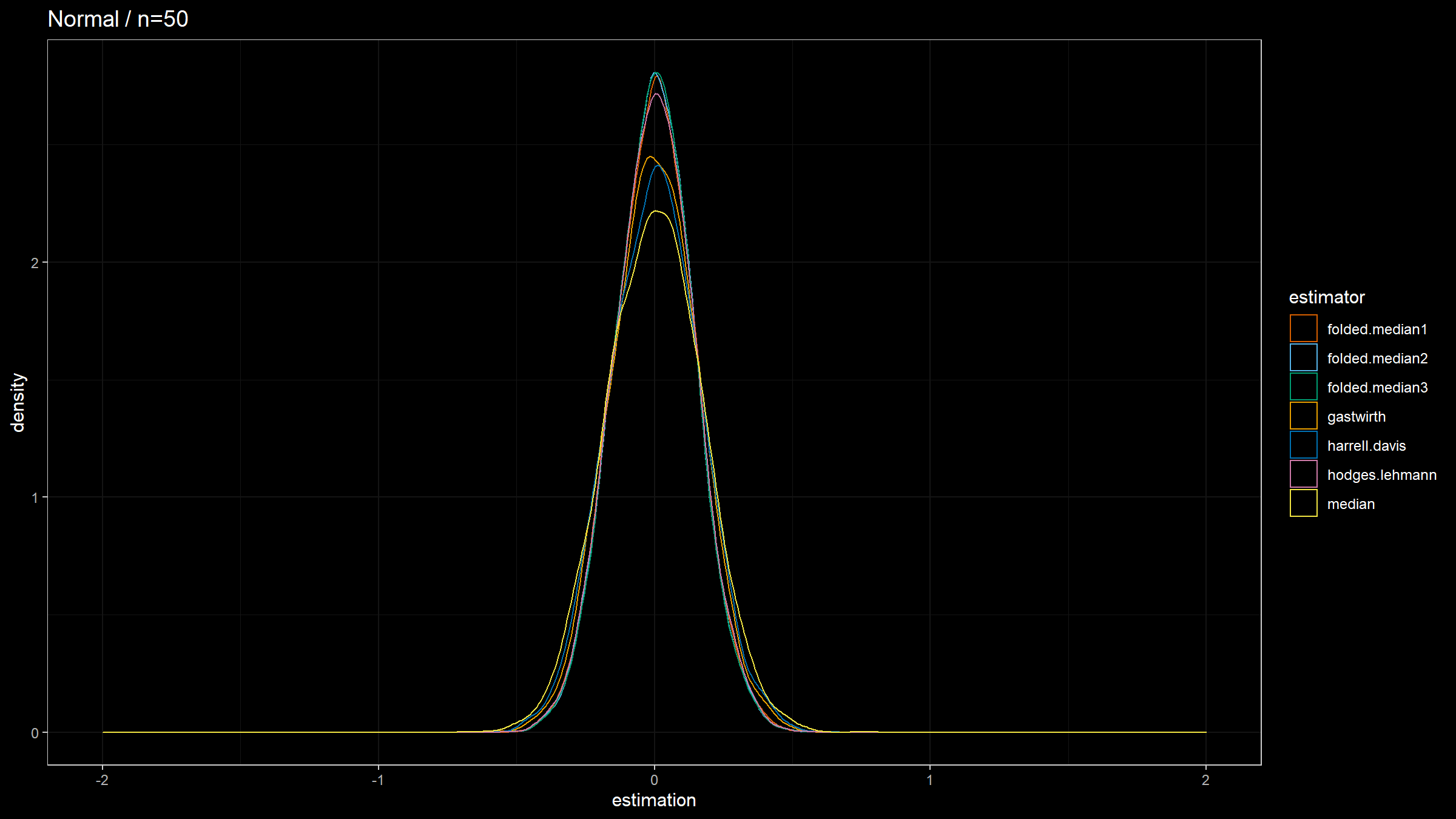
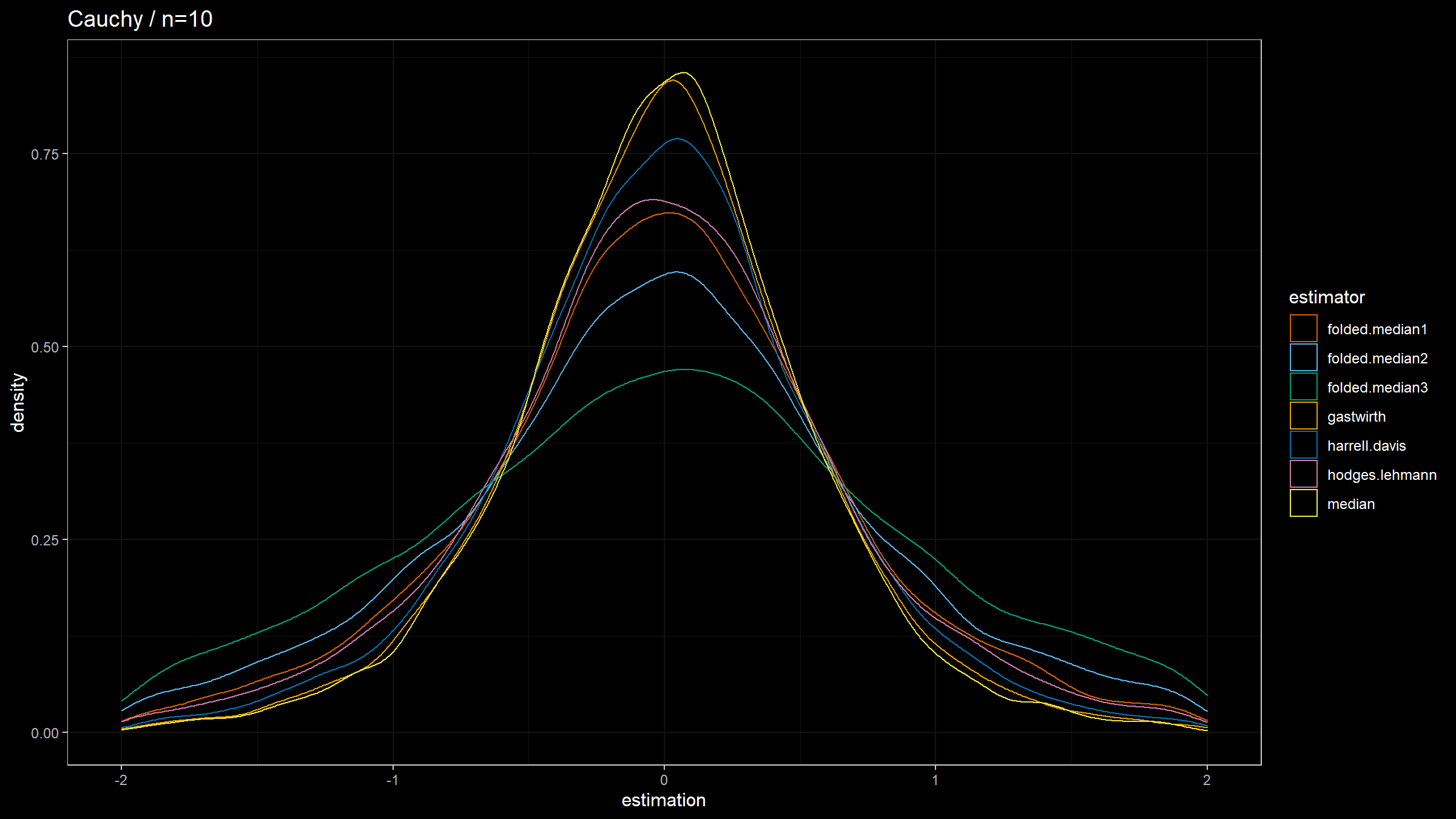
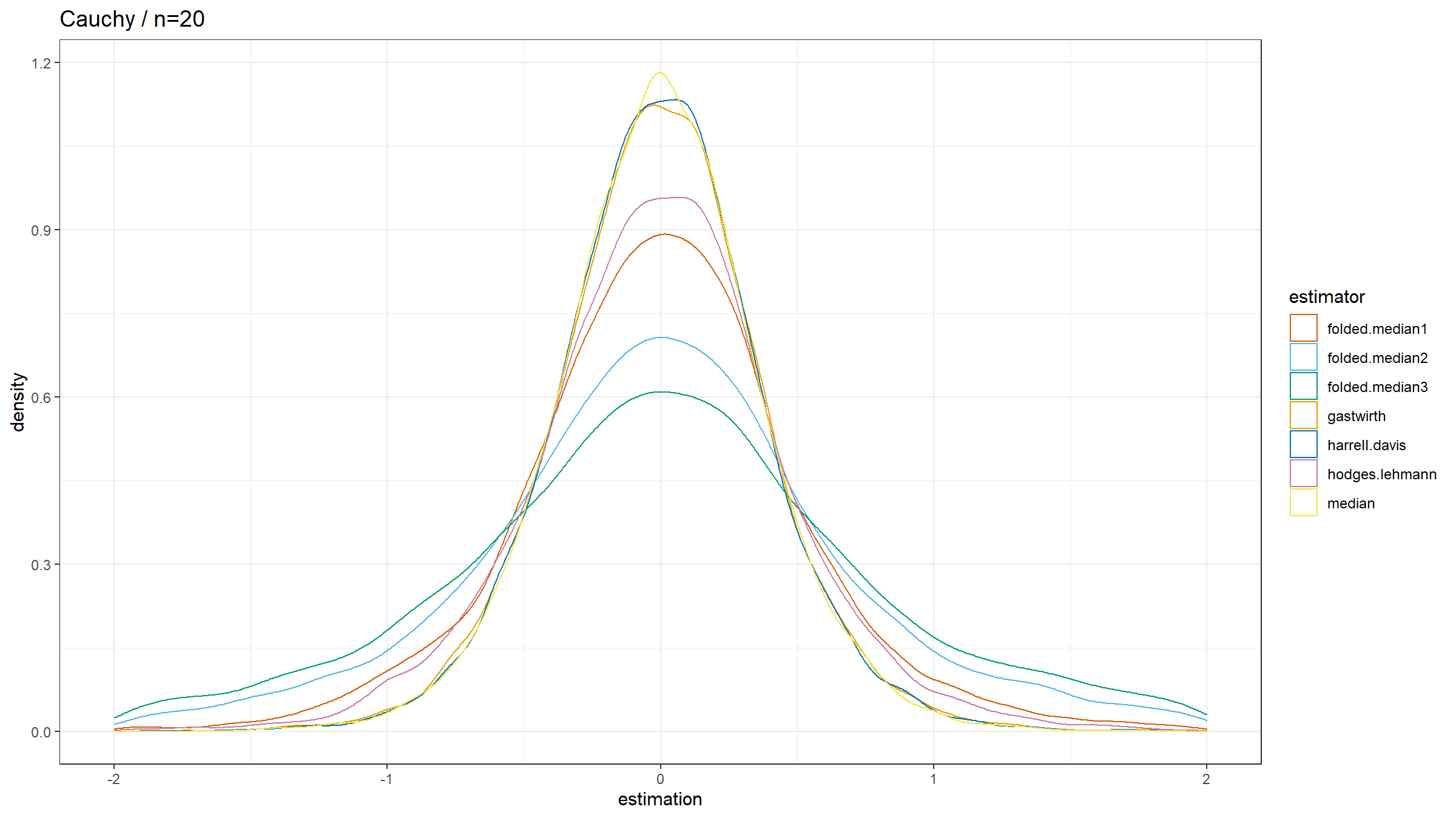
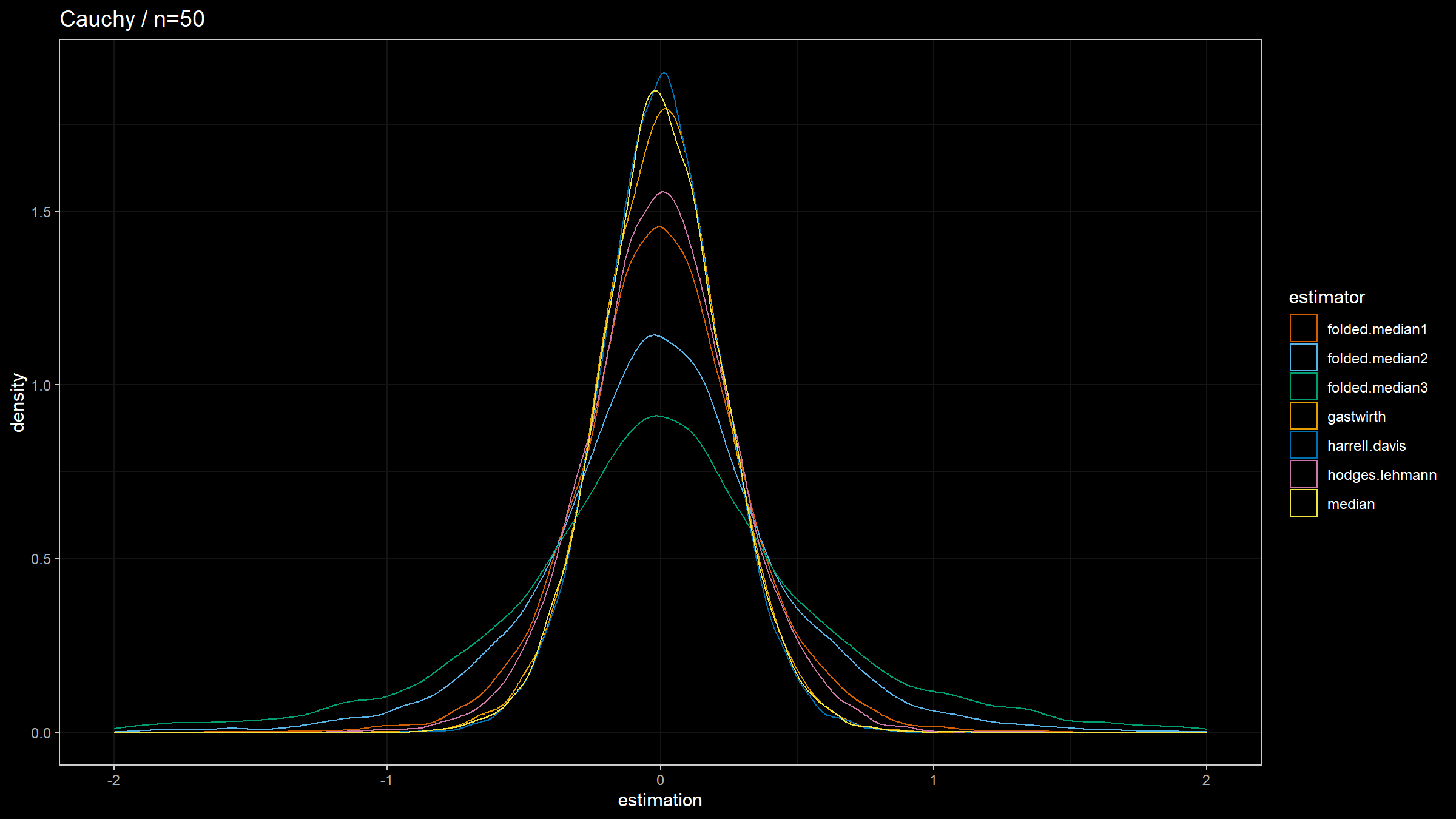
Here are the results:
The observations:
- In the case of the Normal distributions, $Q_{\operatorname{FM*}}$ has the highest statistical efficiency. It’s even more efficient than $Q_{\operatorname{G}}$, $Q_{\operatorname{HD}}$, and $Q_{\operatorname{HL}}$.
- In the case of the Cauchy distribution, $Q_{\operatorname{FM*}}$ has the lowest statistical efficiency, showing its poor robustness.
The folded median approach could be practically interesting in some light-tailed cases because of its high efficiency.
References
- Andrews, David F., and Frank R. Hampel. “Robust estimates of location.”. Princeton University Press, 2015.
- Bickel, P. J., and J. L. Hodges Jr. “The asymptotic theory of Galton’s test and a related simple estimate of location.” The Annals of Mathematical Statistics 38, no. 1 (1967): 73-89. DOI: 10.1214/aoms/1177699059
- Hodges, J. L. “Efficiency in Normal Samples and Tolerance of Extreme.” In Proceedings of the Fifth Berkeley Symposium on Mathematical Statistics and Probability: Weather modification, vol. 5, p. 163. Univ of California Press, 1967.
