Gamma effect size powered by the middle non-zero quantile absolute deviation

In previous posts, I covered the concept of the gamma effect size. It’s a nonparametric effect size which is consistent with Cohen’s d under the normal distribution. However, the original definition has drawbacks: this statistic becomes zero if half of the sample elements are equal to each other. Last time, I suggested) a workaround for this problem: we can replace the median absolute deviation by the quantile absolute deviation. Unfortunately, this trick requires parameter tuning: we should choose a proper quantile position to make this approach work. Today I want to suggest a strategy that provides a way to make a generic choice: we can use the middle non-zero quantile absolute deviation.

Recall

First of all, let’s recall the general equation for the gamma effect size for the $p^\textrm{th}$ quantile:

$$ \gamma_p = \frac{Q_p(y) - Q_p(x)}{\operatorname{PMAD}_{xy}} $$

where $Q_p$ is a quantile estimator of the $p^\textrm{th}$ quantile, $\operatorname{PMAD}_{xy}$ is the pooled median absolute deviation:

$$ \operatorname{PMAD}_{xy} = \sqrt{\frac{(n_x - 1) \operatorname{MAD}^2_x + (n_y - 1) \operatorname{MAD}^2_y}{n_x + n_y - 2}}, $$

$\operatorname{MAD}_x$ and $\operatorname{MAD}_y$ are the median absolute deviations of $x$ and $y$:

$$ \operatorname{MAD}_x = C_{n_x} \cdot Q_{0.5}(|x_i - Q_{0.5}(x)|), \quad \operatorname{MAD}_y = C_{n_y} \cdot Q_{0.5}(|y_i - Q_{0.5}(y)|), $$

$C_{n_x}$ and $C_{n_y}$ are consistency constants that makes $\operatorname{MAD}$ a consistent estimator for the standard deviation estimation. They can be chosen based on the used quantile estimators:

• Constants for the traditional quantile estimator
• Constants for the Harrell-Davis quantile estimator
• Constants for the trimmed Harrell-Davis quantile estimator

QAD instead of MAD

The $\operatorname{MAD}$ approach has a severe drawback: if half of the sample elements equal to the $p^\textrm{th}$ quantile, $\operatorname{MAD}$ becomes zero. Thereby, we can’t use the gamma effect size to compare quantile values.

The problem can be solved using the Quantile Absolute Deviation(QAD) around the given quantile:

$$ \operatorname{QAD}_x(p, q) = C_n \cdot Q_q(|x_i - Q_p(x)|) $$

It’s easy to see that the $\operatorname{MAD}$ is just a special case of $\operatorname{QAD}$:

$$ \operatorname{MAD}_x = \operatorname{QAD}_x(0.5, 0.5). $$

By analogy with $\operatorname{MAD}$, we can define the pooled quantile absolute deviation $\operatorname{PQAD}_{xy}$:

$$ \operatorname{PQAD}_{xy}(p, q) = \sqrt{\frac{ (n_x - 1) \operatorname{QAD}^2_x(p, q) + (n_y - 1) \operatorname{QAD}^2_y(p, q)}{n_x + n_y - 2}}, $$

The only problem with the approach is that we have to define $q$.

MNZQAD instead of QAD

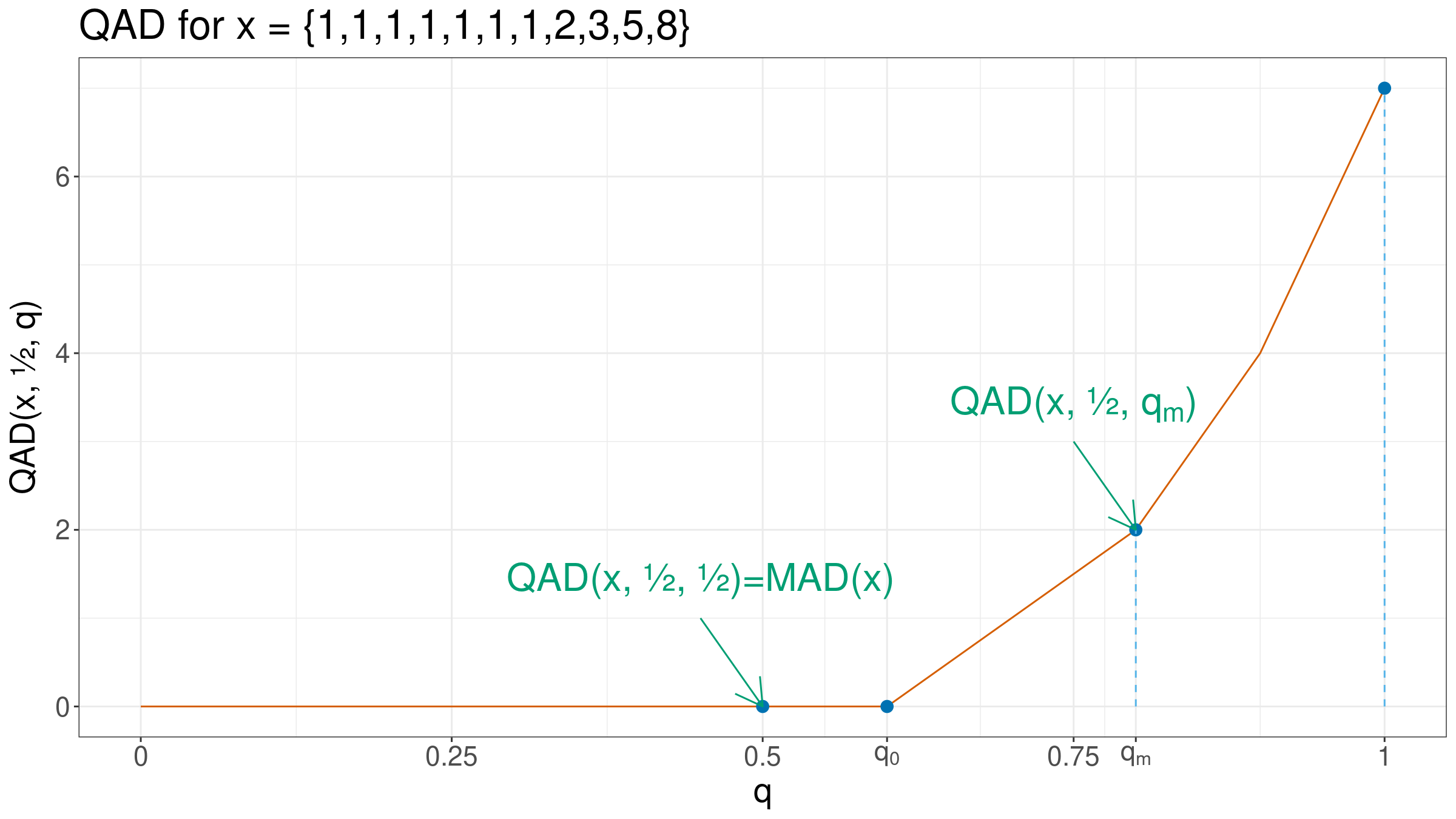
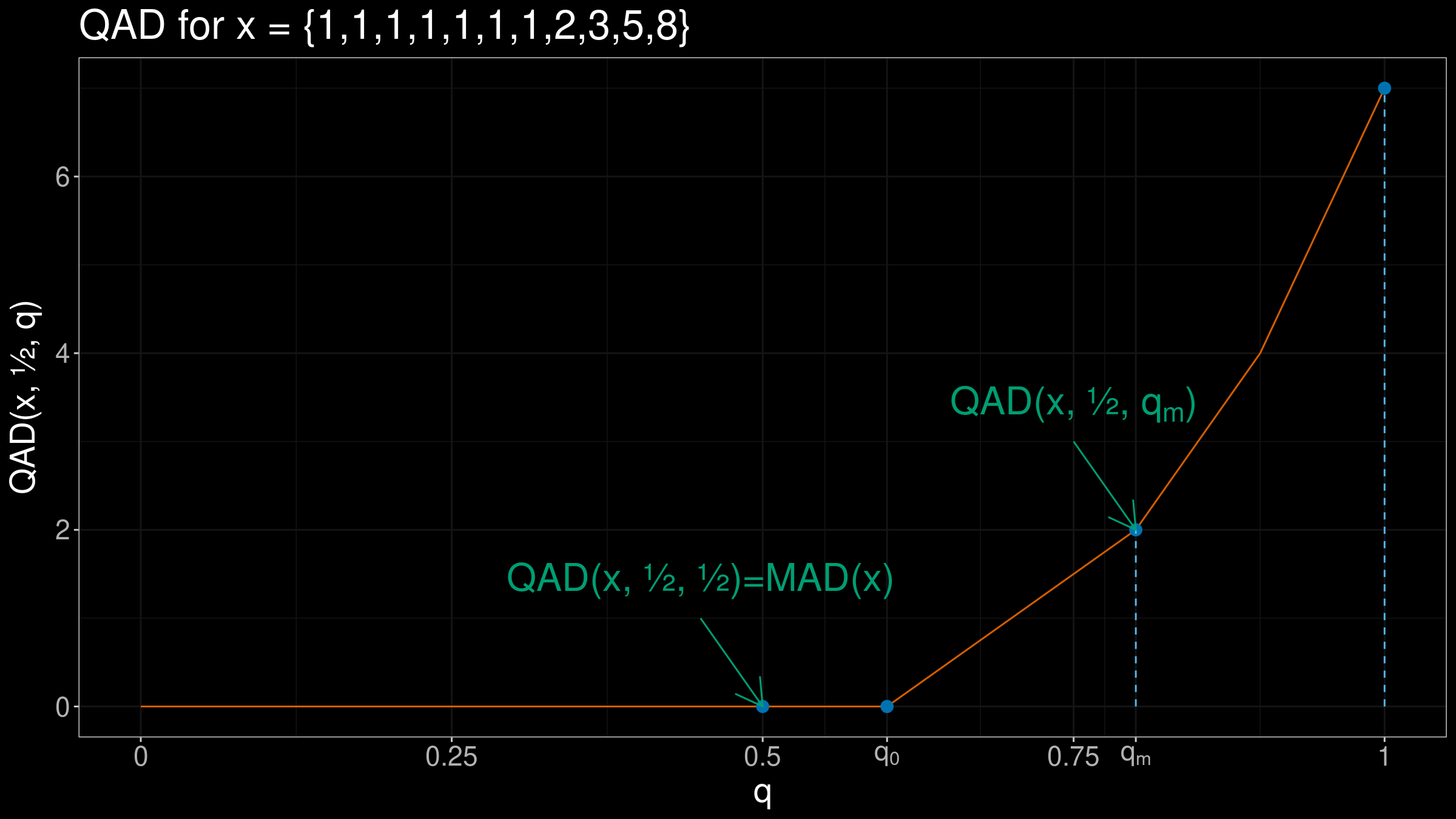
In my previous post, I suggested the idea of the middle non-zero quantile absolute deviation:

$$ \operatorname{MNZQAD(x, p)} = \operatorname{QAD(x, p, q_m)}, $$ $$ q_m = \frac{q_0 + 1}{2}, \quad q_0 = \frac{\max(k - 1, 0)}{n - 1}, \quad k = \sum_{i=1}^n \mathbf{1}_{Q(x, p)}(x_i), $$

where $\mathbf{1}$ is the indicator function:

$$ \mathbf{1}_U(u) = \begin{cases} 1 & \textrm{if}\quad u = U,\\ 0 & \textrm{if}\quad u \neq U. \end{cases} $$

Thus, we peek the middle $q$ values across all $q$ values that gives non-zero $\operatorname{QAD}$:

We can also define a pooled version of $\operatorname{MNZQAD}$:

$$ \operatorname{PMNZQAD}_{xy}(p) = \sqrt{\frac{ (n_x - 1) \operatorname{MNZQAD}^2_x(p) + (n_y - 1) \operatorname{MNZQAD}^2_y(p)}{n_x + n_y - 2}}, $$

With this enchantment, the gamma effect size is always defined for samples with non-zero ranges.