Gastwirth's location estimator
Let $x = \{ x_1, x_2, \ldots, x_n \}$ be a random sample. The Gastwirth’s location estimator is defined as follows:
$$ 0.3 \cdot Q_{⅓}(x) + 0.4 \cdot Q_{½}(x) + 0.3 \cdot Q_{⅔}(x), $$where $Q_p$ is an estimation of the $p^{\textrm{th}}$ quantile (using classic sample quantiles).
This estimator could be quite interesting from a practical point of view. On the one hand, it’s robust (the breakdown point ⅓) and it has better statistical efficiency than the classic sample median. On the other hand, it has better computational efficiency than other robust and statistical efficient measures of location like the Harrell-Davis median estimator or the Hodges-Lehmann median estimator.
In this post, we conduct a short simulation study that shows its behavior for the standard Normal distribution and the Cauchy distribution.
Simulation study
Let’s conduct the following simulation:
- Enumerate different samples sizes $n = \{ 5, 10, 20 \}$
- Enumerate different location estimators: Gastwirth’s location estimator $Q_{\operatorname{G}}$, the sample median $Q_{\operatorname{SM}}$, the Harrell-Davis median estimator $Q_{\operatorname{HD}}$, and the Hodges-Lehmann median estimator $Q_{\operatorname{HL}}$.
- Enumerate different distributions: the standard Normal distribution, the standard Cauchy distribution
- For each sample size, estimator, and distribution, generate $30\,000$ random samples of the given size from the given distribution and calculate the location estimation using the given estimator.
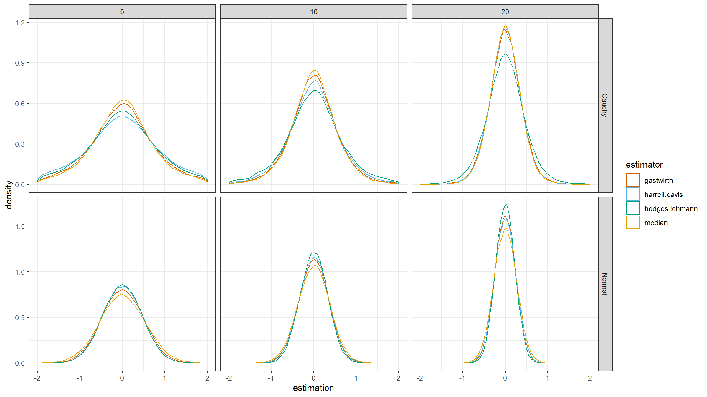
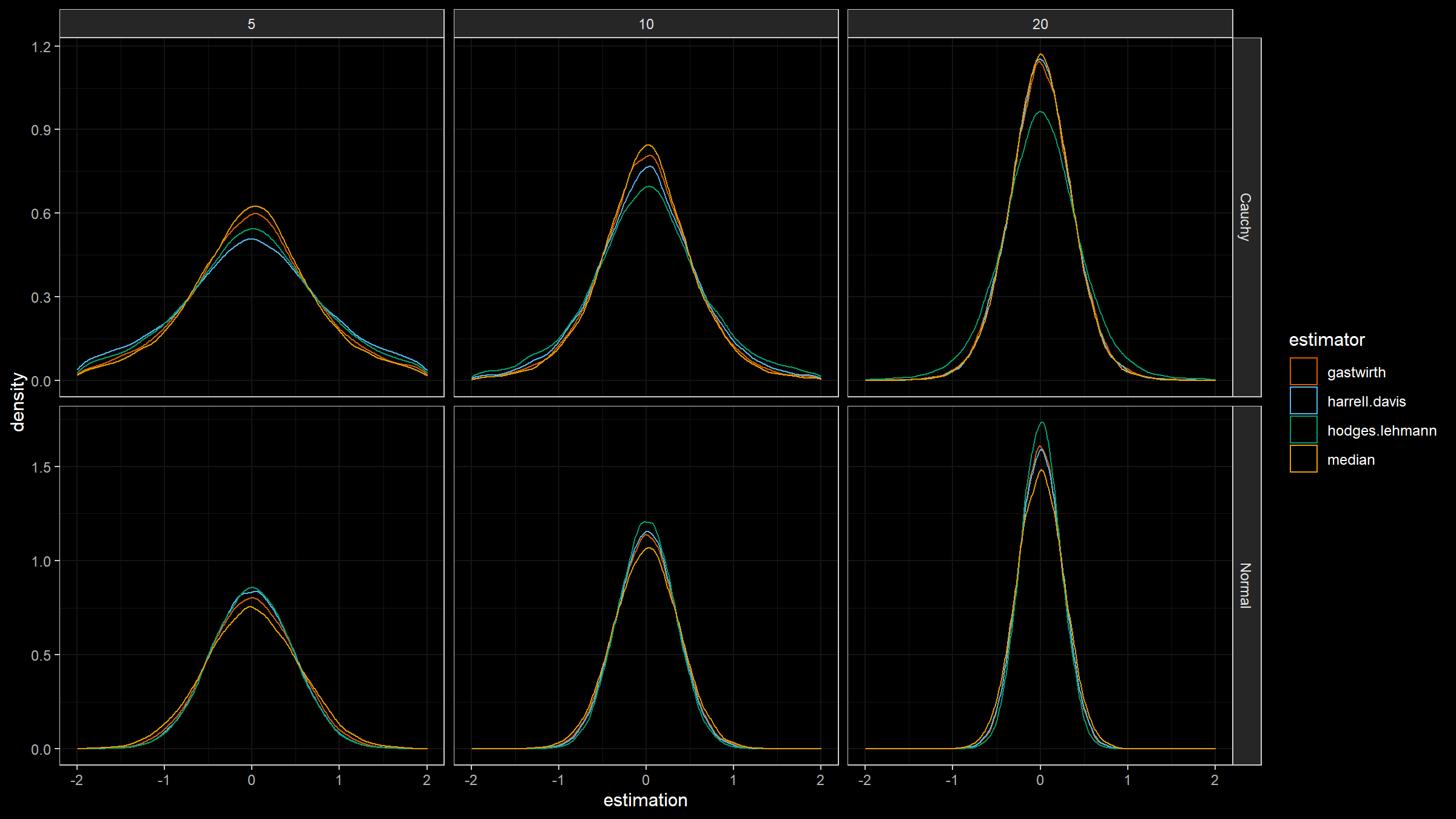
- Draw the corresponding density plots for the obtained estimation using Sheather & Jones method and the normal kernel.
Here are the results:
Based on this plot, we can do the following observations:
- For the standard Normal distribution (light-tailed), $Q_{\operatorname{G}}$ is better than $Q_{\operatorname{SM}}$, but worse than $Q_{\operatorname{HD}}$ and $Q_{\operatorname{HL}}$.
- For the standard Cauchy distribution (heavy-tailed), $Q_{\operatorname{G}}$ is worse than $Q_{\operatorname{SM}}$, but better than $Q_{\operatorname{HD}}$ and $Q_{\operatorname{HL}}$.
Of course, a more sophisticated study is required for reliable conclusions, but this simulation shows that Gastwirth’s location estimator is quite promising. It provides an interesting trade-off between statistical efficiency, computational efficiency, and robustness. It could be useful if we want to improve the statistical efficiency of the sample median for the light-tailed cases, keeping a decent breakdown point (⅓) and computational efficiency.
References
- Gastwirth, Joseph L. “On robust procedures.” Journal of the American Statistical Association 61, no. 316 (1966): 929-948. DOI:10.1080/01621459.1966.10482185
- Patel, K. R., Mudholkar, G. S., & Fernando, J. L. I. (1988). Student’s t Approximations for Three Simple Robust Estimators. Journal of the American Statistical Association, 83(404), 1203. DOI:10.2307/2290158
- Gogoi, Chikhla Jun, and Bipin Gogoi. “Estimation of Location Parameter Using Adaptive and Some Other Methods.” Journal of Management (JOM) 7, no. 2 (2020).
- Andrews, David F., and Frank R. Hampel. “Robust estimates of location.”. Princeton University Press, 2015.
- Gastwirth’s location estimator by Ron Pearson

