Sensitivity curve of the Harrell-Davis quantile estimator, Part 1
The Harrell-Davis quantile estimator is an efficient replacement for the traditional quantile estimator, especially in the case of light-tailed distributions. Unfortunately, it is not robust: its breakdown point is zero. However, the breakdown point is not the only descriptor of robustness. While the breakdown point describes the portion of the distribution that should be replaced by arbitrary large values to corrupt the estimation, it does not describe the actual impact of finite outliers. The arithmetic mean also has the breakdown point of zero, but the practical robustness of the mean and the Harrell-Davis quantile estimator are not the same. The Harrell-Davis quantile estimator is an L-estimator that assigns extremely low weights to sample elements near the tails (especially, for reasonably large sample sizes). Therefore, the actual impact of potential outliers is not so noticeable. In this post, we use the standardized sensitivity curve to evaluate this impact.
The classic Harrell-Davis quantile estimator (see A new distribution-free quantile estimator
By Frank E Harrell, C E Davis
·
1982harrell1982) is defined as follows:
where $I_t(\alpha, \beta)$ is the regularized incomplete beta function, $\alpha = (n+1)p$, $\;\beta = (n+1)(1-p)$. In this post we consider the Harrell-Davis median estimator $Q_{\operatorname{HD}}(0.5)$.
The standardized sensitivity curve (SC) of an estimator $\hat{\theta}$ is given by
$$ \operatorname{SC}_n(x_0) = \frac{ \hat{\theta}_{n+1}(x_1, x_2, \ldots, x_n, x_0) - \hat{\theta}_n(x_1, x_2, \ldots, x_n) }{1 / (n + 1)} $$Thus, the SC shows the standardized change of the estimator value for situation, when we add a new element $x_0$ to an existing sample $\mathbf{x} = \{ x_1, x_2, \ldots, x_n \}$. In the context of this post, we perform simulations using the standard normal distribution given by its quantile function $\Phi^{-1}$. Following the approach from [Maronna2019, Section 3.1], we define the sample $\mathbf{x}$ as
$$ \mathbf{x} = \Bigg\{ \Phi^{-1}\Big(\frac{1}{n+1}\Big), \Phi^{-1}\Big(\frac{2}{n+1}\Big), \ldots, \Phi^{-1}\Big(\frac{n}{n+1}\Big) \Bigg\} $$Now let’s explore the SC values for different sample sizes for $x_0 \in [-100; 100]$:
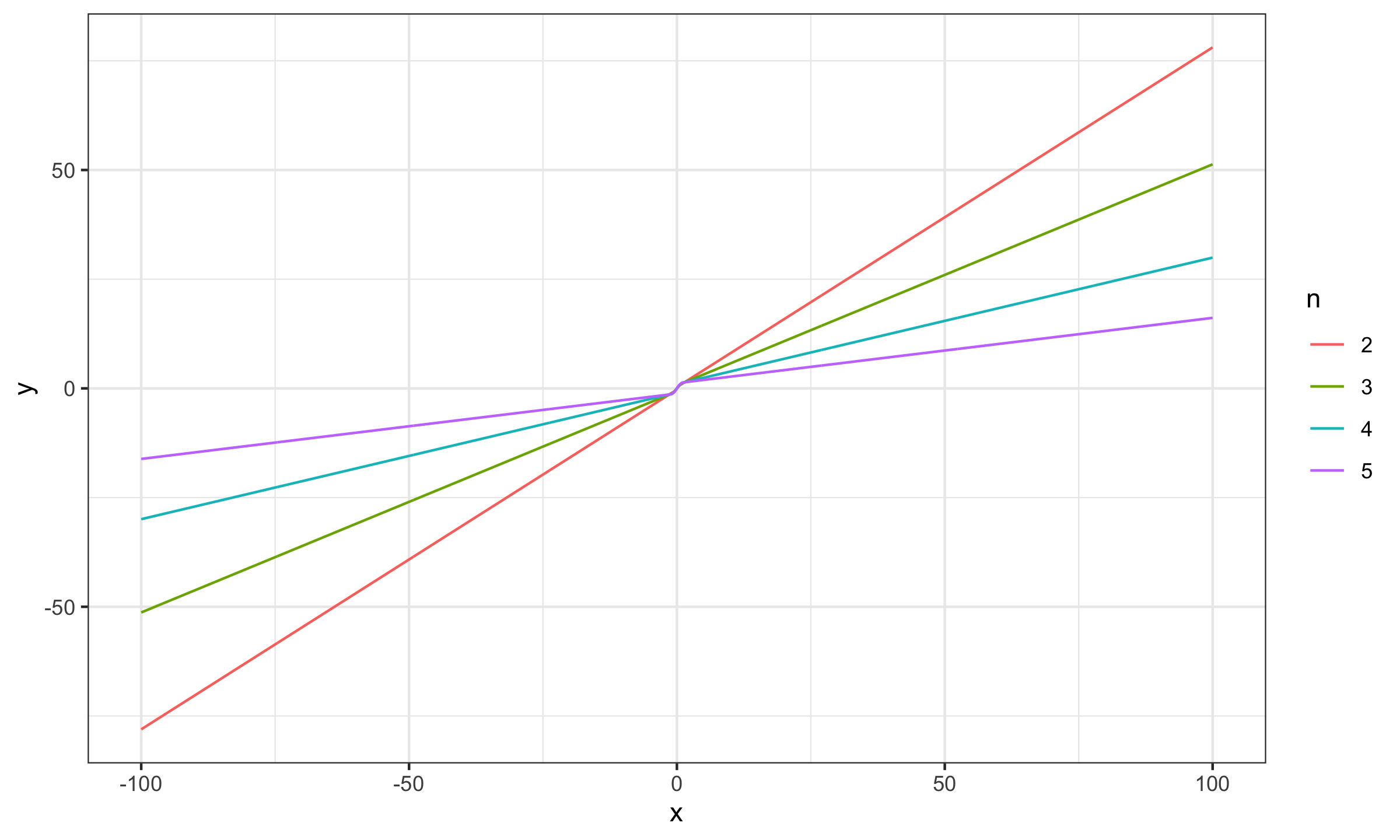
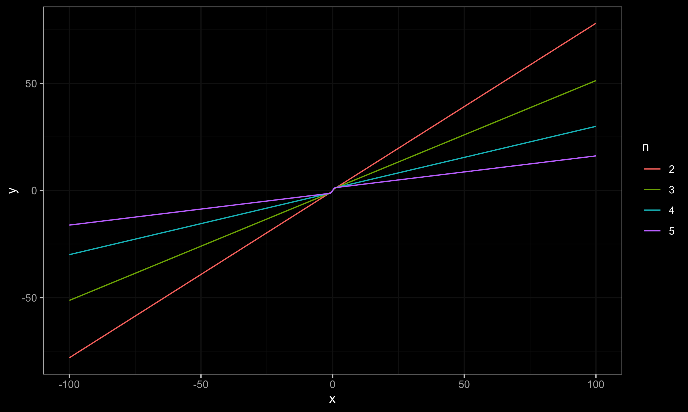
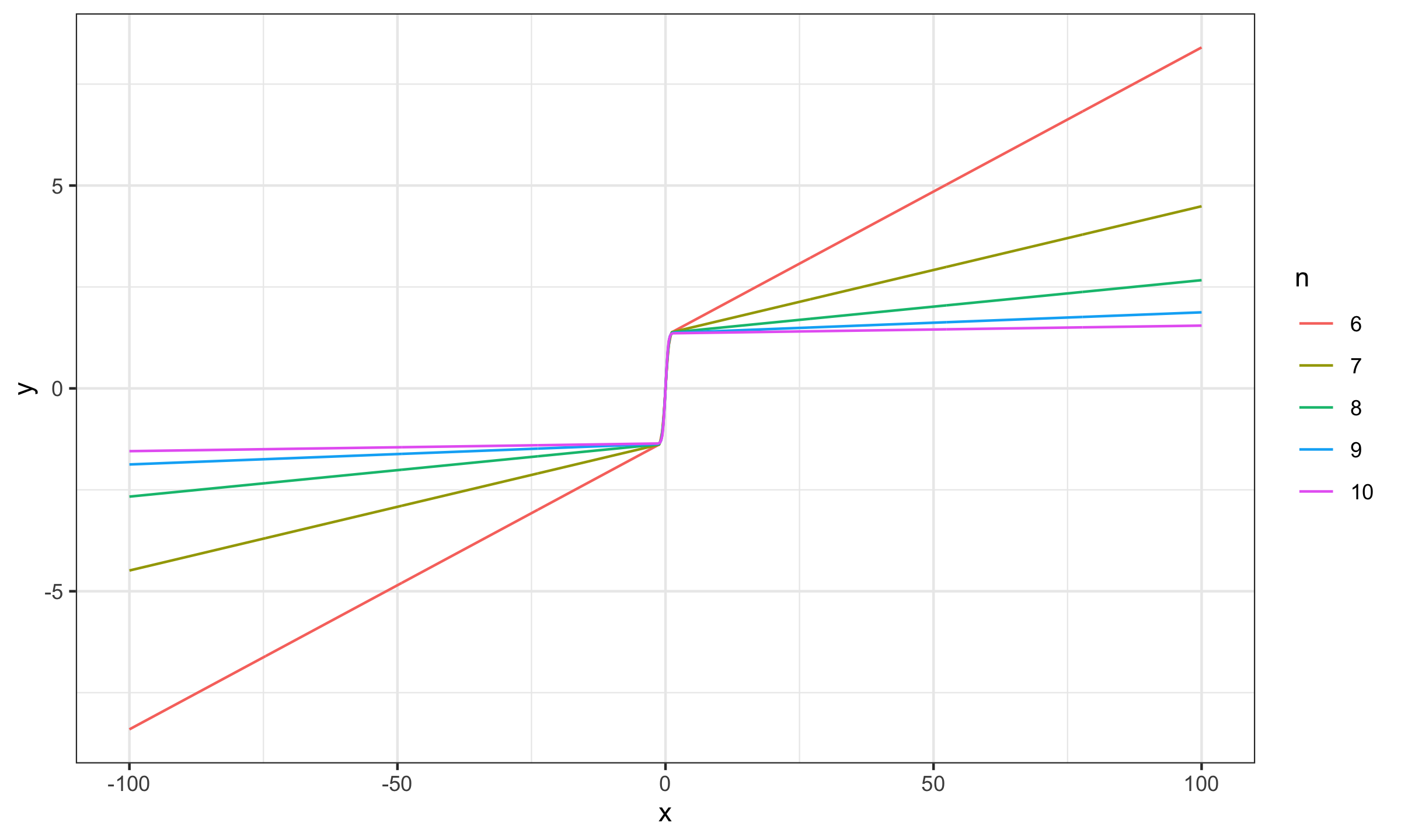

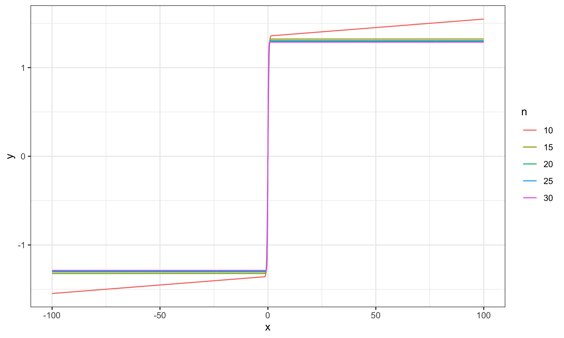
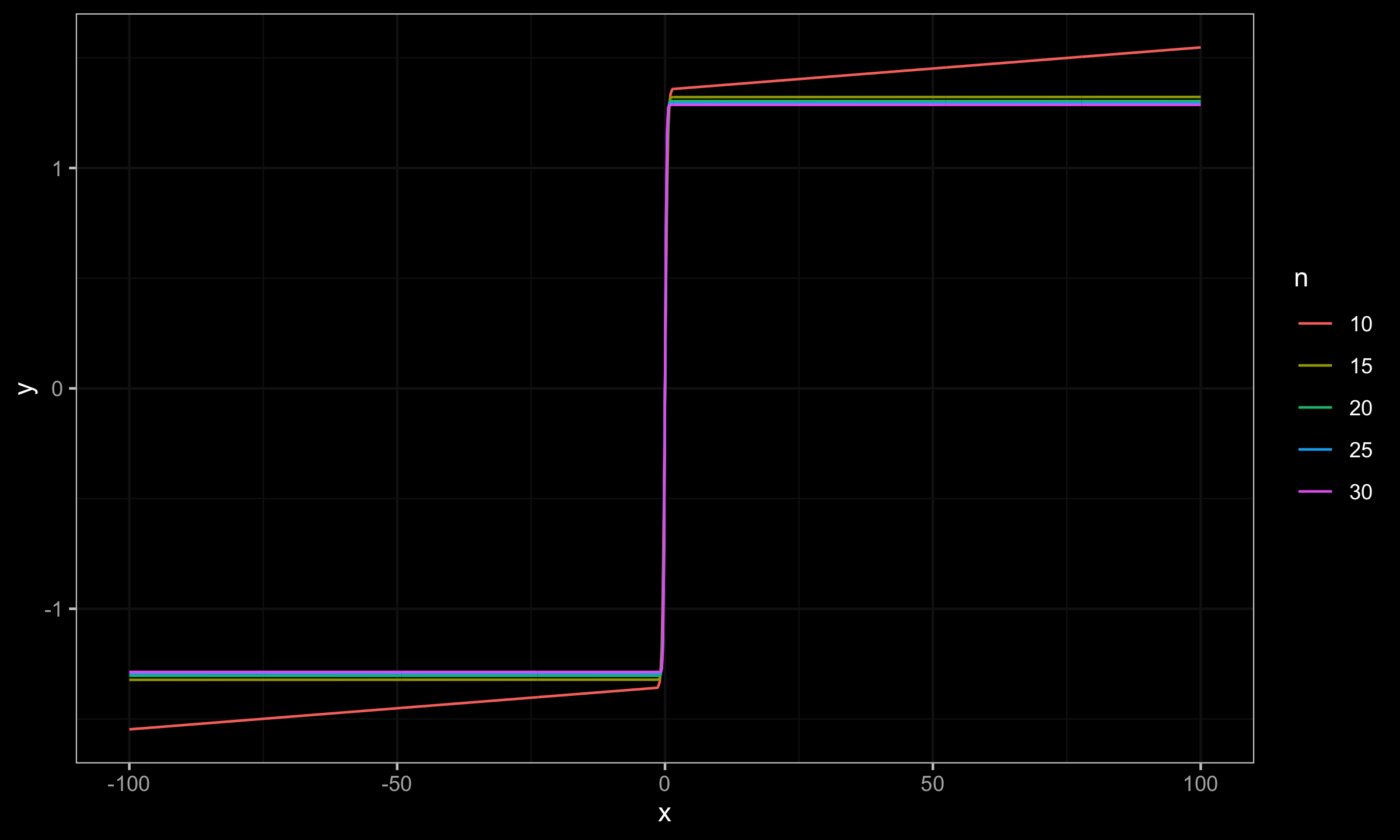
As we can see, for $n \geq 15$ the actual impact of $x_0$ is negligible, which makes the Harrell-Davis median estimator a practically reasonable choice.
References
- [Harrell1982]
Harrell, F.E. and Davis, C.E., 1982. A new distribution-free quantile estimator. Biometrika, 69(3), pp.635-640.
https://doi.org/10.2307/2335999 - [Maronna2019]
Maronna, Ricardo A., R. Douglas Martin, Victor J. Yohai, and Matías Salibián-Barrera. Robust statistics: theory and methods (with R). John Wiley & Sons, 2019.