Sensitivity curve of the Harrell-Davis quantile estimator, Part 3
In the previous posts (1, 2), I have explored the sensitivity curves of the Harrell-Davis quantile estimator on the normal distribution, the exponential distribution, and the Cauchy distribution. In this post, I build these sensitivity curves for some additional distributions.
The classic Harrell-Davis quantile estimator (see A new distribution-free quantile estimator
By Frank E Harrell, C E Davis
·
1982harrell1982) is defined as follows:
where $I_t(\alpha, \beta)$ is the regularized incomplete beta function, $\alpha = (n+1)p$, $\;\beta = (n+1)(1-p)$. In this post we consider the Harrell-Davis median estimator $Q_{\operatorname{HD}}(0.5)$.
The standardized sensitivity curve (SC) of an estimator $\hat{\theta}$ is given by
$$ \operatorname{SC}_n(x_0) = \frac{ \hat{\theta}_{n+1}(x_1, x_2, \ldots, x_n, x_0) - \hat{\theta}_n(x_1, x_2, \ldots, x_n) }{1 / (n + 1)} $$Thus, the SC shows the standardized change of the estimator value for situation, when we add a new element $x_0$ to an existing sample $\mathbf{x} = \{ x_1, x_2, \ldots, x_n \}$. In the context of this post, we perform simulations using the different distributions given by their quantile functions that we denote as $F^{-1}$. Following the approach from [Maronna2019, Section 3.1], we define the sample $\mathbf{x}$ as
$$ \mathbf{x} = \Bigg\{ F^{-1}\Big(\frac{1}{n+1}\Big), F^{-1}\Big(\frac{2}{n+1}\Big), \ldots, F^{-1}\Big(\frac{n}{n+1}\Big) \Bigg\} $$Now let’s explore the SC values for different sample sizes for $x_0 \in [-100; 100]$.
Distributions
We consider the following distributions:
| Distribution | Support | Skewness | Tailness |
|---|---|---|---|
Uniform(a=0, b=1) | $[0;1]$ | Symmetric | Light-tailed |
Triangular(a=0, b=2, c=1) | $[0;2]$ | Symmetric | Light-tailed |
Triangular(a=0, b=2, c=0.2) | $[0;2]$ | Right-skewed | Light-tailed |
Beta(a=2, b=4) | $[0;1]$ | Right-skewed | Light-tailed |
Beta(a=2, b=10) | $[0;1]$ | Right-skewed | Light-tailed |
Normal(m=0, sd=1) | $(-\infty;+\infty)$ | Symmetric | Light-tailed |
Weibull(scale=1, shape=2) | $[0;+\infty)$ | Right-skewed | Light-tailed |
Student(df=3) | $(-\infty;+\infty)$ | Symmetric | Light-tailed |
Gumbel(loc=0, scale=1) | $(-\infty;+\infty)$ | Right-skewed | Light-tailed |
Exp(rate=1) | $[0;+\infty)$ | Right-skewed | Light-tailed |
Cauchy(x0=0, gamma=1) | $(-\infty;+\infty)$ | Symmetric | Heavy-tailed |
Pareto(loc=1, shape=0.5) | $[1;+\infty)$ | Right-skewed | Heavy-tailed |
Pareto(loc=1, shape=2) | $[1;+\infty)$ | Right-skewed | Heavy-tailed |
LogNormal(mlog=0, sdlog=1) | $(0;+\infty)$ | Right-skewed | Heavy-tailed |
LogNormal(mlog=0, sdlog=2) | $(0;+\infty)$ | Right-skewed | Heavy-tailed |
LogNormal(mlog=0, sdlog=3) | $(0;+\infty)$ | Right-skewed | Heavy-tailed |
Weibull(shape=0.3) | $[0;+\infty)$ | Right-skewed | Heavy-tailed |
Weibull(shape=0.5) | $[0;+\infty)$ | Right-skewed | Heavy-tailed |
Frechet(shape=1) | $(0;+\infty)$ | Right-skewed | Heavy-tailed |
Frechet(shape=3) | $(0;+\infty)$ | Right-skewed | Heavy-tailed |
Sensitivity curves
Here are the results of numerical simulations:

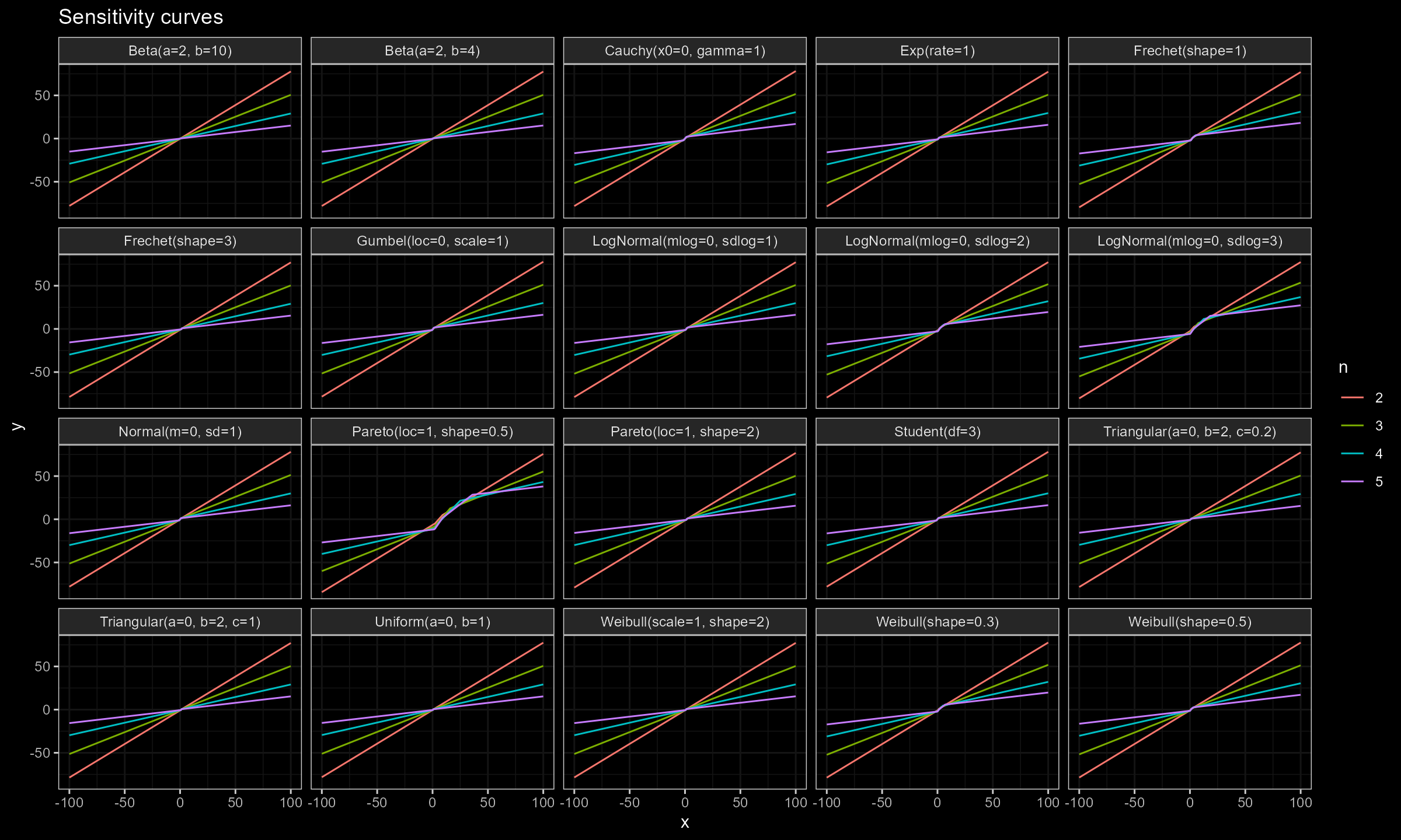
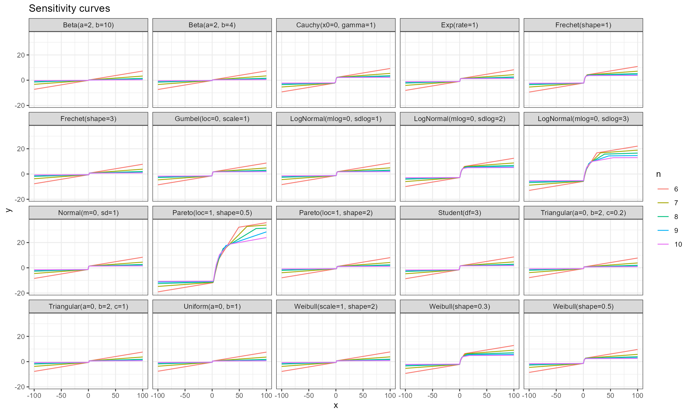
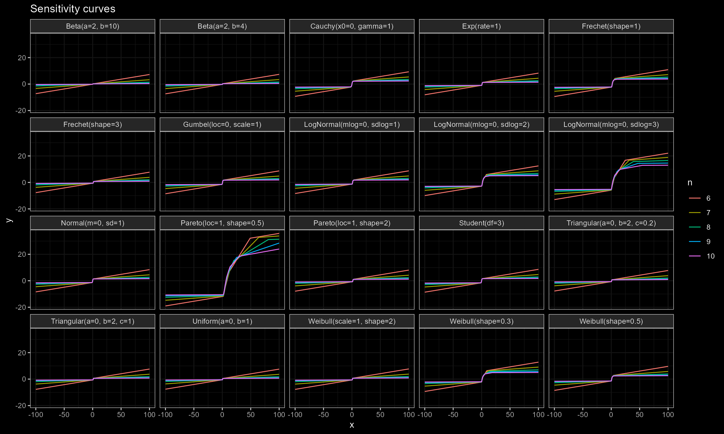
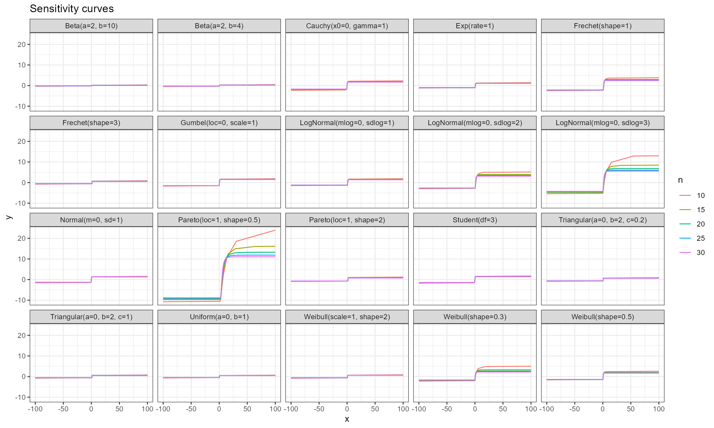

Conclusion
As we can see, for $n \geq 15$ the actual impact of $x_0$ is negligible, which makes the Harrell-Davis median estimator a practically reasonable choice regardless of the distribution. However, we should be careful with heavy distributions like the Pareto or LogNormal distributions.
References
- [Harrell1982]
Harrell, F.E. and Davis, C.E., 1982. A new distribution-free quantile estimator. Biometrika, 69(3), pp.635-640.
https://doi.org/10.2307/2335999 - [Maronna2019]
Maronna, Ricardo A., R. Douglas Martin, Victor J. Yohai, and Matías Salibián-Barrera. Robust statistics: theory and methods (with R). John Wiley & Sons, 2019.