Comparing the efficiency of the Harrell-Davis, Sfakianakis-Verginis, and Navruz-Özdemir quantile estimators
In the previous posts, I discussed the statistical efficiency of different quantile estimators (Efficiency of the Harrell-Davis quantile estimator and Efficiency of the winsorized and trimmed Harrell-Davis quantile estimators).
In this post, I continue this research and compare the efficiency of the Harrell-Davis quantile estimator, the Sfakianakis-Verginis quantile estimators, and the Navruz-Özdemir quantile estimator.
Simulation design
The relative efficiency value depends on five parameters:
- Target quantile estimator
- Baseline quantile estimator
- Estimated quantile $p$
- Sample size $n$
- Distribution
In this case study, we are going to compare three target quantile estimators:
(1) The Harrell-Davis (HD) quantile estimator (
A new distribution-free quantile estimator
By Frank E Harrell, C E Davis
·
1982harrell1982):
where $I_t(a, b)$ denotes the regularized incomplete beta function, $x_{(i)}$ is the $i^\textrm{th}$ order statistics.
(2) The Sfakianakis-Verginis (SV) quantile estimators (
A new family of nonparametric quantile estimators
By Michael E Sfakianakis, Dimitris G Verginis
·
2008sfakianakis2008):
where $B_i = B(i; n, p)$ is probability mass function of the binomial distribution $B(n, p)$, $X_{(i)}$ are order statistics of sample $X$.
(3) The Navruz-Özdemir (NO) quantile estimator (
A new quantile estimator with weights based on a subsampling approach
By G"ozde Navruz, A Firat "Ozdemir
·
2020navruz2020):
where $B_i = B(i; n, p)$ is probability mass function of the binomial distribution $B(n, p)$, $X_{(i)}$ are order statistics of sample $X$.
The conventional baseline quantile estimator in such simulations is
the traditional quantile estimator that is defined as
a linear combination of two subsequent order statistics.
To be more specific, we are going to use the Type 7 quantile estimator from the Hyndman-Fan classification or
HF7 (
Sample Quantiles in Statistical Packages
By Rob J Hyndman, Yanan Fan
·
1996hyndman1996).
It can be expressed as follows (assuming one-based indexing):
Thus, we are going to estimate the relative efficiency of HD, SV1, SV2, SV3, and NO quantile estimators comparing to the traditional quantile estimator HF7. For the $p^\textrm{th}$ quantile, the relative efficiency of the target quantile estimator $Q_\textrm{Target}$ can be calculated as the ratio of the estimator mean squared errors ($\textrm{MSE}$):
$$ \textrm{Efficiency}(p) = \dfrac{\textrm{MSE}(Q_{HF7}, p)}{\textrm{MSE}(Q_\textrm{Target}, p)} = \dfrac{\operatorname{E}[(Q_{HF7}(p) - \theta(p))^2]}{\operatorname{E}[(Q_\textrm{Target}(p) - \theta(p))^2]} $$where $\theta(p)$ is the true value of the $p^\textrm{th}$ quantile. The $\textrm{MSE}$ value depends on the sample size $n$, so it should be calculated independently for each sample size value.
Finally, we should choose the distributions for sample generation. I decided to choose 4 light-tailed distributions and 4 heavy-tailed distributions
| distribution | description |
|---|---|
| Beta(2,10) | Beta distribution with a=2, b=10 |
| U(0,1) | Uniform distribution on [0;1] |
| N(0,1^2) | Normal distribution with mu=0, sigma=1 |
| Weibull(1,2) | Weibull distribution with scale=1, shape=2 |
| Cauchy(0,1) | Cauchy distribution with location=0, scale=1 |
| Pareto(1, 0.5) | Pareto distribution with xm=1, alpha=0.5 |
| LogNormal(0,3^2) | Log-normal distribution with mu=0, sigma=3 |
| Exp(1) + Outliers | 95% of exponential distribution with rate=1 and 5% of uniform distribution on [0;10000] |
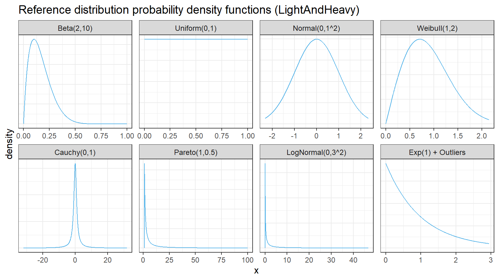
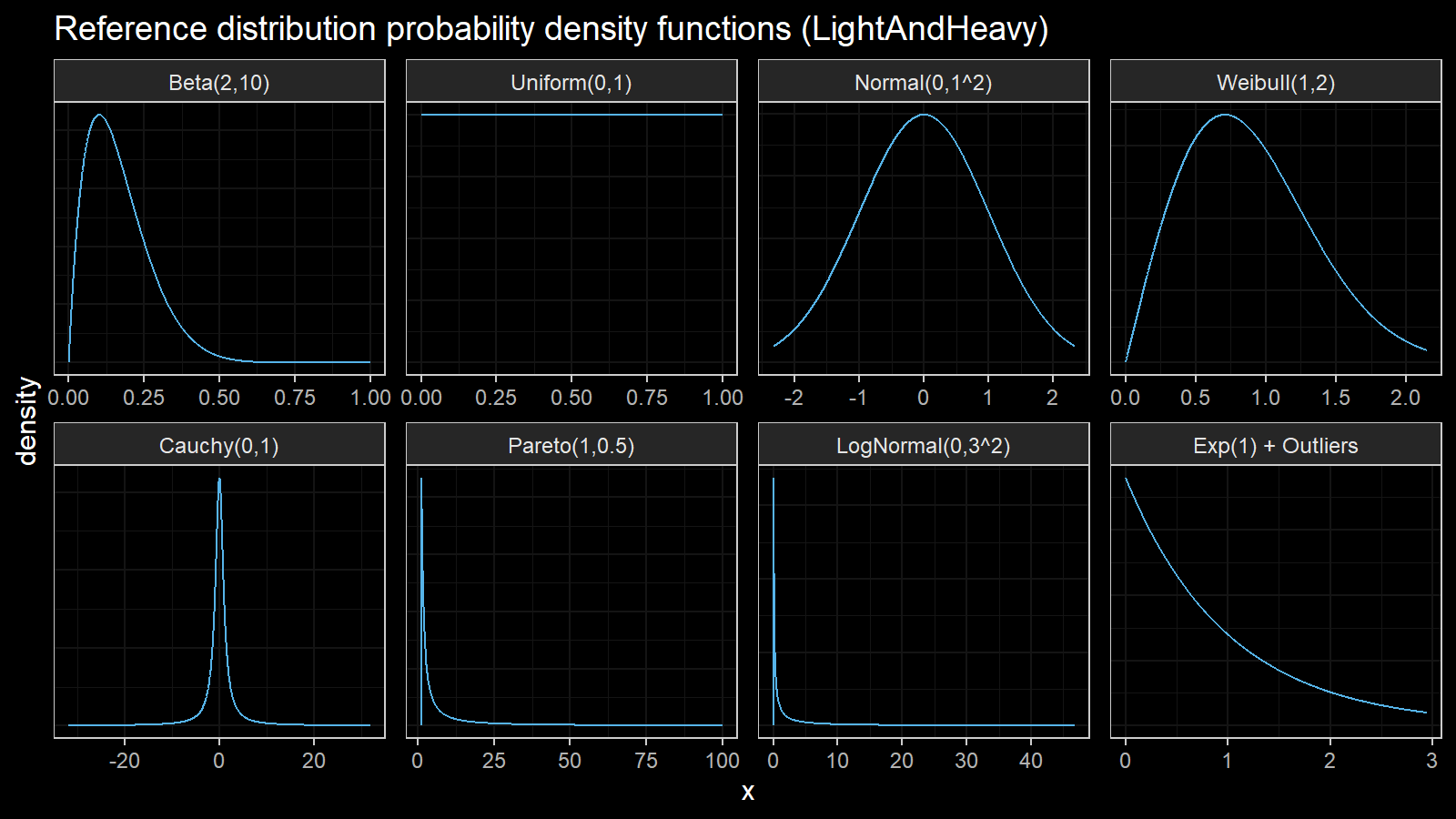
Here are the probability density functions of these distributions:
For each distribution, we are going to do the following:
- Enumerate all the percentiles and calculate the true percentile value $\theta(p)$ for each distribution
- Enumerate different sample sizes (from 3 to 40)
- Generate a bunch of random samples, estimate the percentile values using all estimators, calculate the relative efficiency of all target quantile estimators quantile estimator.
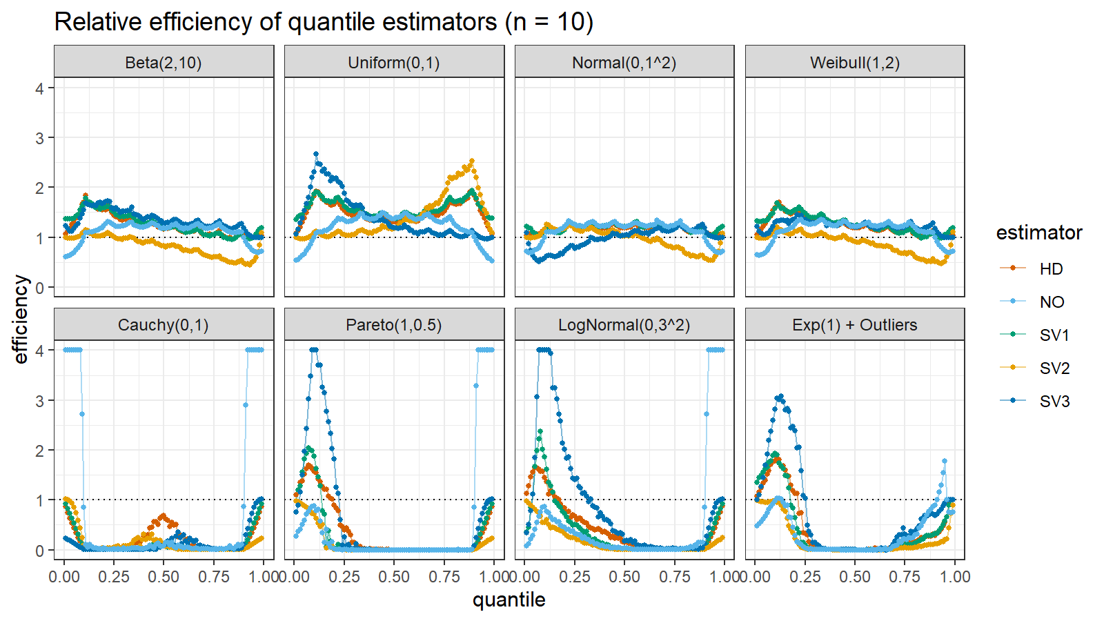
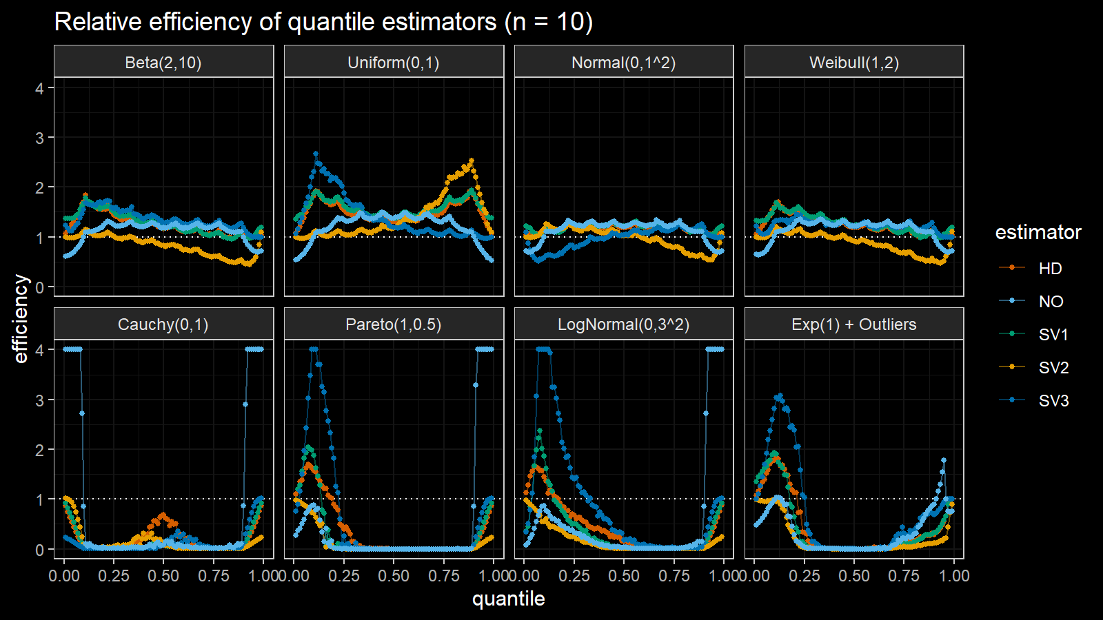
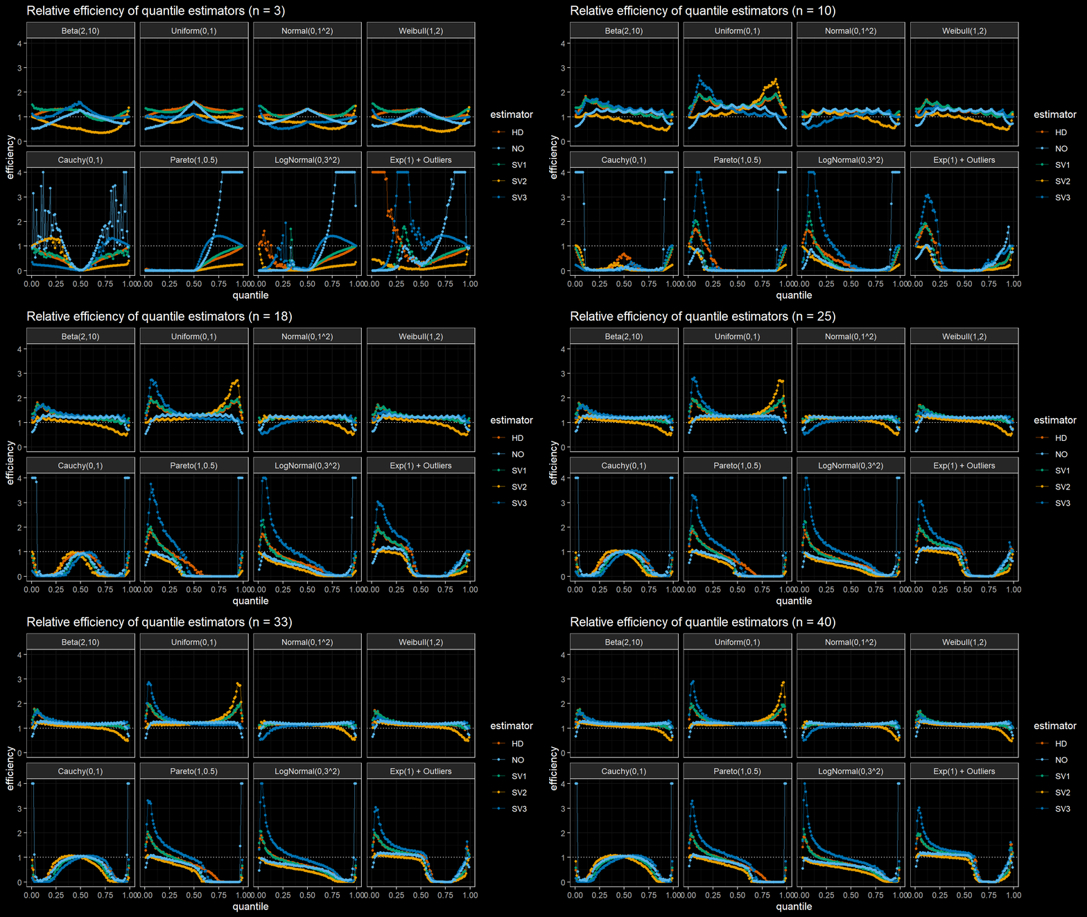
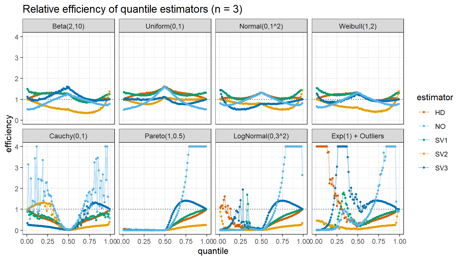
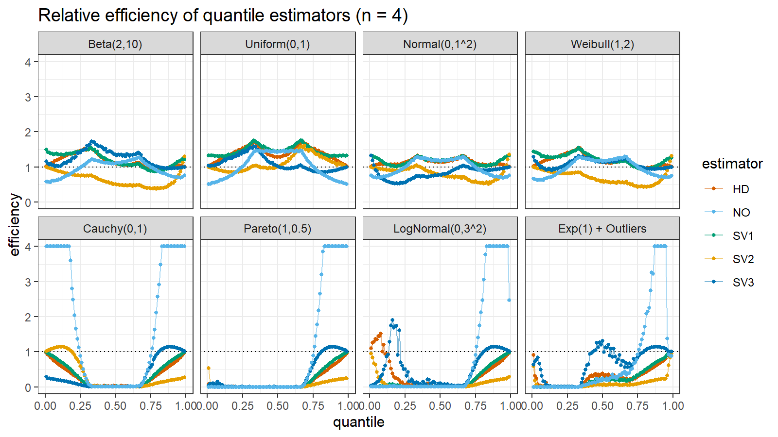
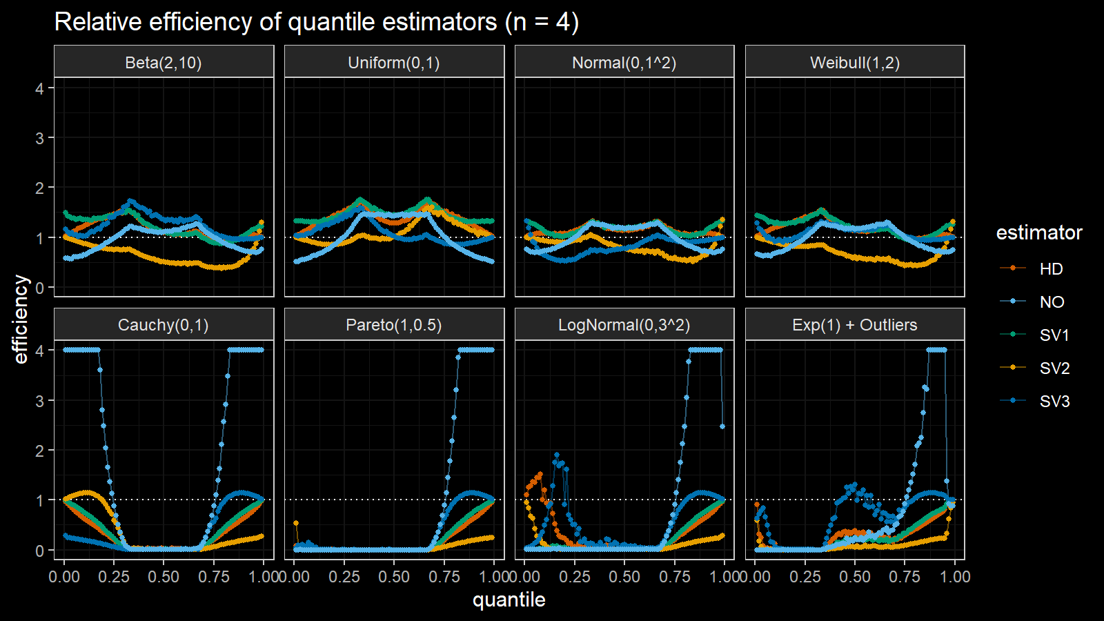
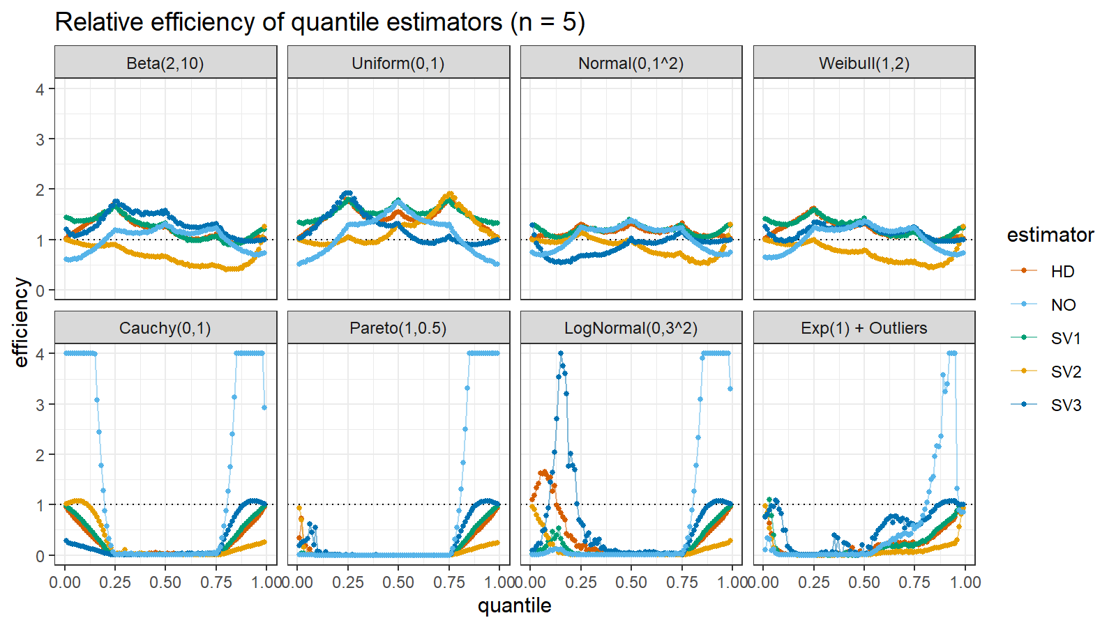
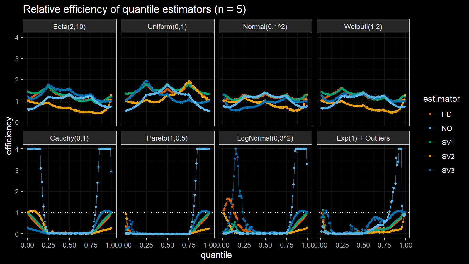
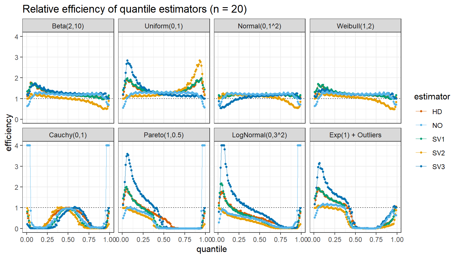
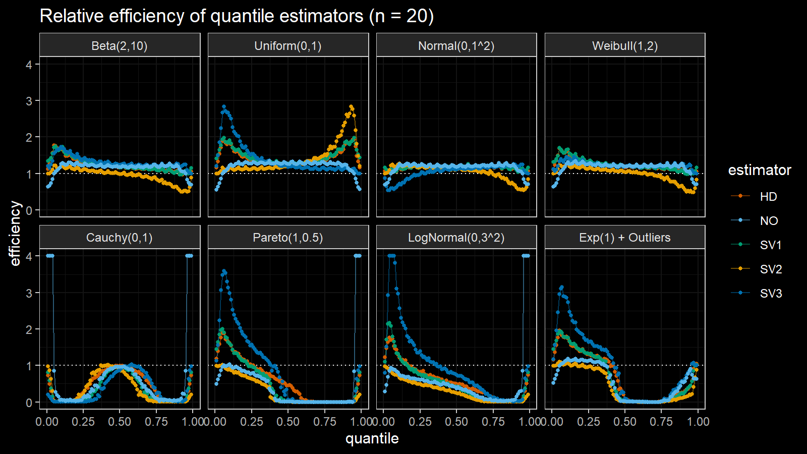
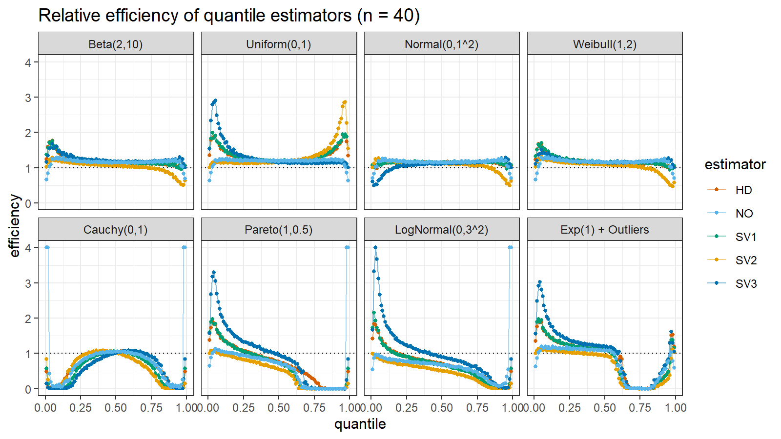
Here are the results of the simulation:
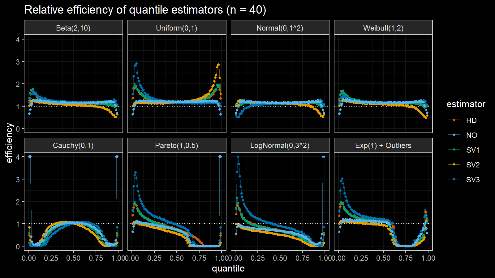
Here are the static charts for some of the $n$ values:
Conclusion
Based on the above simulation, we could draw the following observations:
- The HD quantile estimator seems to be a good choice for unknown distribution.
- The SV3 quantile estimator provides good efficiency for the high-density area of heavy-tailed right-skewed distributions.
- By analogy, we can assume that the SV2 quantile estimator provides good efficiency for the high-density area of heavy-tailed left-skewed distributions.
- The NO quantile estimator provides good efficiency for the low-density area of heavy-tailed distributions on small samples.
References
- [Harrell1982]
Harrell, F.E. and Davis, C.E., 1982. A new distribution-free quantile estimator. Biometrika, 69(3), pp.635-640.
https://doi.org/10.2307/2335999 - [Sfakianakis2008]
Sfakianakis, Michael E., and Dimitris G. Verginis. “A new family of nonparametric quantile estimators.” Communications in Statistics—Simulation and Computation® 37, no. 2 (2008): 337-345.
https://doi.org/10.1080/03610910701790491 - [Navruz2020]
Navruz, Gözde, and A. Fırat Özdemir. “A new quantile estimator with weights based on a subsampling approach.” British Journal of Mathematical and Statistical Psychology 73, no. 3 (2020): 506-521.
https://doi.org/10.1111/bmsp.12198 - [Hyndman1996]
Hyndman, R. J. and Fan, Y. 1996. Sample quantiles in statistical packages, American Statistician 50, 361–365.
https://doi.org/10.2307/2684934
