Efficiency of the Harrell-Davis quantile estimator

One of the most essential properties of a quantile estimator is its efficiency. In simple words, the efficiency describes the estimator accuracy. The Harrell-Davis quantile estimator is a good option to achieve higher efficiency. However, this estimator may provide lower efficiency in some special cases. In this post, we will conduct a set of simulations that show the actual efficiency numbers. We compare different distributions (symmetric and right-skewed, heavy-tailed and light-tailed), quantiles, and sample sizes.

Simulation design

The relative efficiency value depends on five parameters:

• Target quantile estimator
• Baseline quantile estimator
• Estimated quantile $p$
• Sample size $n$
• Distribution

Our target quantile estimator is the Harrell-Davis quantile estimator or HDQE (harrell1982).

$$ Q_{HD}(p) = \sum_{i=1}^{n} W_{i} \cdot x_{(i)}, \quad W_{i} = I_{i/n}(a, b) - I_{(i-1)/n}(a, b), \quad a = p(n+1),\; b = (1-p)(n+1) $$

where $I_t(a, b)$ denotes the regularized incomplete beta function, $x_{(i)}$ is the $i^\textrm{th}$ order statistics.

The conventional baseline quantile estimator in such simulations is the traditional quantile estimator that is defined as a linear combination of two subsequent order statistics. To be more specific, we are going to use the Type 7 quantile estimator from the Hyndman-Fan classification or HF7QE (hyndman1996). It can be expressed as follows (assuming one-based indexing):

$$ Q_{HF7}(p) = x_{(\lfloor h \rfloor)}+(h-\lfloor h \rfloor)(x_{(\lfloor h \rfloor+1)})-x_{(\lfloor h \rfloor)},\quad h = (n-1)p+1. $$

Thus, we are going to estimate the relative efficiency of HDQE comparing to the traditional quantile estimator HF7QE. For the $p^\textrm{th}$ quantile, the relative efficiency can be calculated as the ratio of the estimator mean squared errors ($\textrm{MSE}$):

$$ \textrm{Efficiency}(p) = \dfrac{\textrm{MSE}(Q_{HF7}, p)}{\textrm{MSE}(Q_{HD}, p)} = \dfrac{\operatorname{E}[(Q_{HF7}(p) - \theta(p))^2]}{\operatorname{E}[(Q_{HD}(p) - \theta(p))^2]} $$

where $\theta(p)$ is the true value of the $p^\textrm{th}$ quantile. The $\textrm{MSE}$ value depends on the sample size $n$, so it should be calculated independently for each sample size value.

Finally, we should choose the distributions for sample generation. Initially, I wanted to repeat the numerical experiment from harrell1982 (Section 3). The authors used the generalized lambda distribution which is defined by its quantile function:

$$ F^{-1}(p) = \mu + \sigma (p^a - (1-p)^b) $$

They states that they used $\mu = 0$, $\sigma = 1$, and $a, b$ form the following table:

Case	a	b	Description
(a)	1	1	Light-tailed symmetric
(b)	0.1349	0.1349	Normal-like
(c)	-0.1359	-0.1359	Very heavy-tailed symmetric, like t-distribution with 5 degrees of freedom
(d)	-1	-1	Cauchy-like
(e)	0.0251	0.0953	Medium-tailed asymmetric
(f)	0	0.0004	Exponential-like

Unfortunately, there are problems with this table. Cases (c) and (d) are invalid because we can’t use negative values of $a$ and $b$ with a positive value of $\sigma$: such combination produces decreasing quantile function. Even if we flip the sign of $\sigma$, the suggested distributions are not close to their descriptions. For example, (b) doesn’t look like the normal distribution, (d) doesn’t look like the Cauchy distribution, (f) doesn’t look like the exponential distribution.

So, I decided to build my own set of distributions and evaluate the efficiency of the Harrell-Davis quantile estimator in each case.

For each distribution, we are going to do the following:

• Enumerate all the percentiles and calculate the true percentile value $\theta(p)$ for each distribution
• Enumerate different sample sizes (from 3 to 60)
• Generate a bunch of random samples, estimate the percentile values using two estimators, calculate the relative efficiency of the Harrell-Davis quantile estimator.

Let’s look at the results for different groups of distributions.

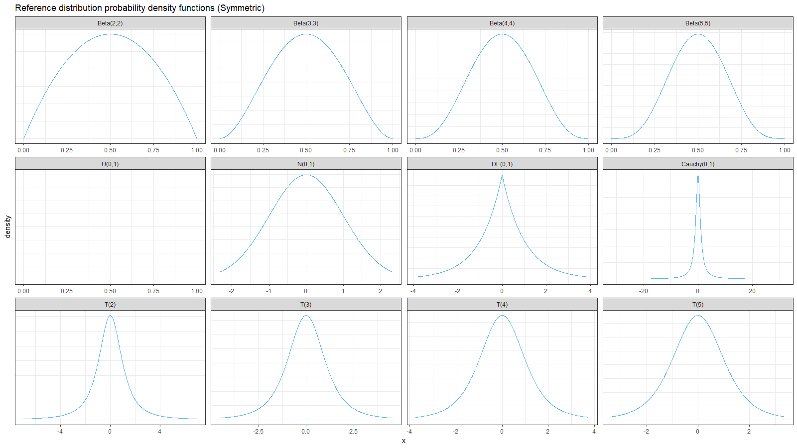
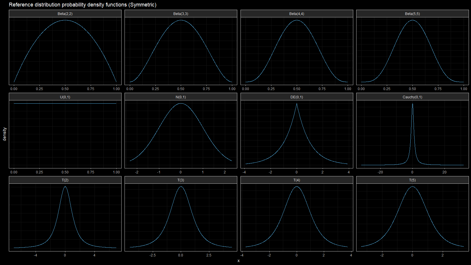
Symmetric

We start with symmetric distributions from the following list:

distribution	description
Beta(2,2)	Beta distribution with a=b=2
Beta(3,3)	Beta distribution with a=b=3
Beta(4,4)	Beta distribution with a=b=4
Beta(5,5)	Beta distribution with a=b=4
U(0,1)	Uniform distribution on [0;1]
N(0,1)	Normal with mu=0, sigma=1
DE(0,1)	Laplace (double exponential) with mu=0, b=1
Cauchy(0,1)	Cauchy distribution with location=0, scale=1
T(2)	Student’s t with 2 degrees of freedom
T(3)	Student’s t with 3 degrees of freedom
T(4)	Student’s t with 4 degrees of freedom
T(5)	Student’s t with 5 degrees of freedom

Below you can find the density plots of these distributions and an animation that shows the relative efficiency for different sample sizes.

Here we can make a few observations:

• For light-tailed distributions (beta, uniform, normal), the Harrell-Davis quantile estimator is more efficient than the traditional one for all the percentiles.
• For heavy-tailed distribution (Laplace, Cauchy, Student), the Harrell-Davis quantile estimator is more efficient in the middle of the distribution and less efficient on the tails.

Unimodal right-skewed

Next, we consider different right skewed distributions: exponential, beta (with $a < b$), Gumbel, Pareto, Weibull, Frechet, log-normal:

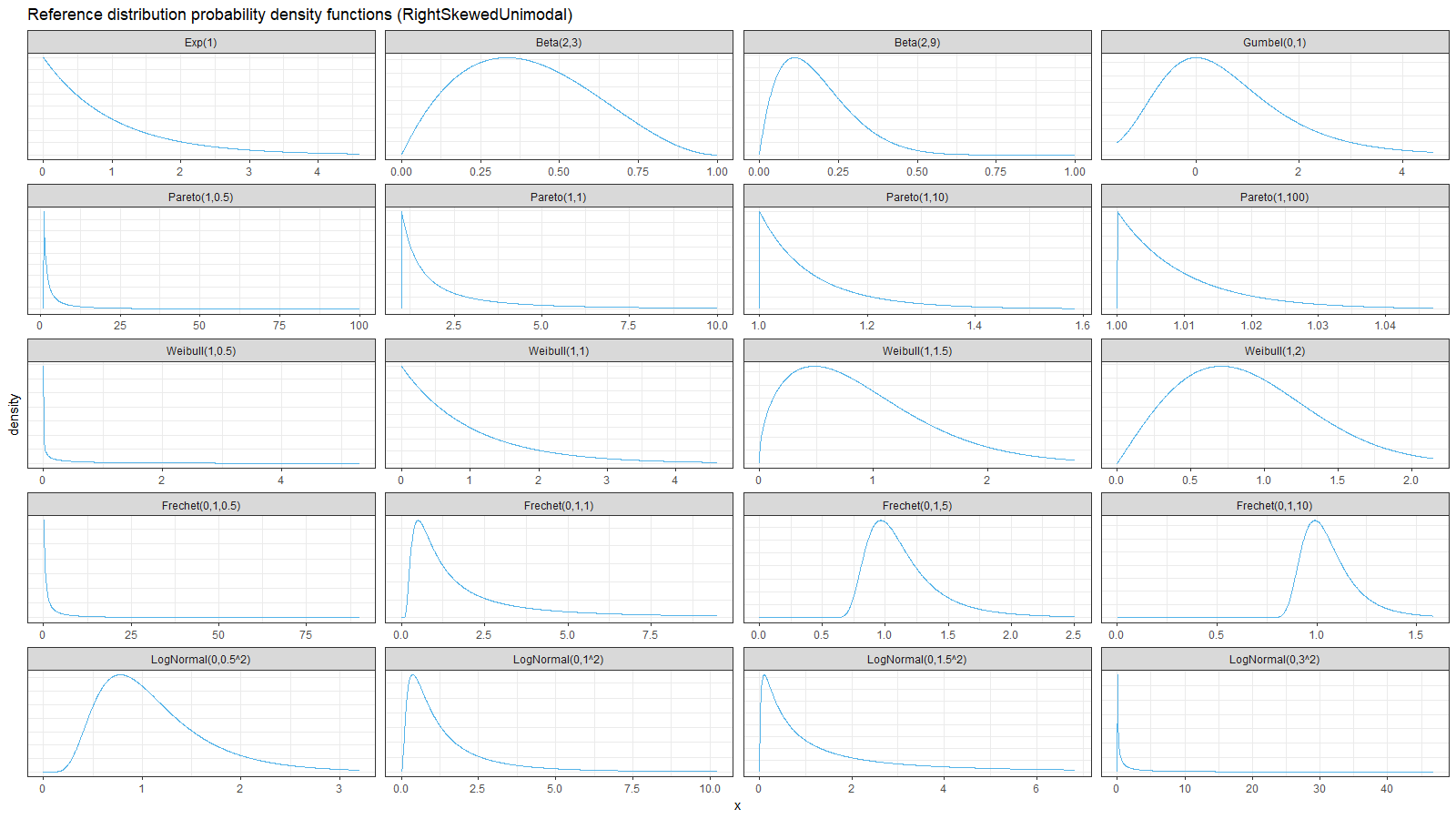
On the left side of these plots, the Harrell-Davis quantile estimator is always more efficient than the traditional one. However, it’s not so efficient on the tails. The region of the inefficiency depends on the heaviness of the tail and on the sample size.

In the case of distributions closed to the light-tailed case (exponential, Gumbel(0, 1), beta, Pareto with large $\alpha$, Weibull with the shape parameter greater than 1, Frechet with the shape parameter greater than 10, log-normal with $\sigma < 0.5$), HDQE is quite efficient. For small sample sizes (e.g., $n=3$), it’s efficient for $p \in [0, 0.5]$. For medium-size samples (e.g., $n=60$), it’s efficient for $p \in [0, 0.85]$

In the case of heavy-tailed distributions, HDQE is not so efficient. For extremely heavy-tailed cases (e.g. log-normal with $\sigma = 3$), HDQE could be efficient only for $p \in [0, 0.2]$ on samples of any size.

Bimodal right-skewed

For each distribution from the previous section, let’s build a mixture from the original distribution and the original distribution shifted by 10. Thus, we get a set of bimodal right-skewed distributions:

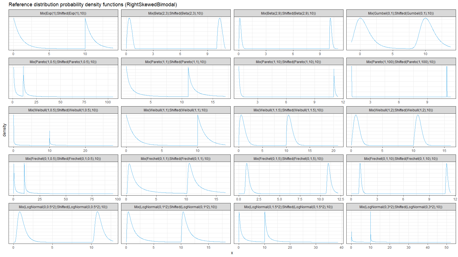
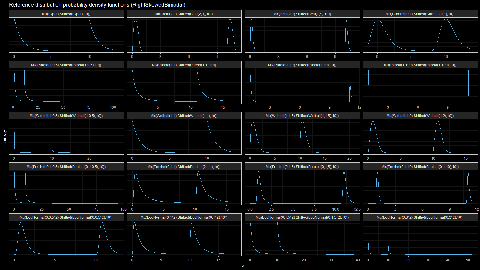
Here we can observe two inefficient areas. The first one is on the tail, as in the previous section. The second one is between modes of the given bimodal distributions.

Synthetic Latency by Brendan Gregg

Finally, let’s consider a set of synthetic latency distribution by Brendan Gregg (the origin can be found here). We are going to work with the following distributions (notation Mix(D1|W1;D2|W2) means a mixture of distribution D1 with weight W1 and distribution D2 with weight W2):

• 0: uniform narrow
  Uniform(500,1500)
• 1: uniform wide
  Uniform(0,3000)
• 2: uniform outliers
  Mix(Uniform(500,1500)|0.99;Uniform(1500,10000)|0.01)
• 100: unimodal normal narrow
  Normal(1000,100^2)
• 101: unimodal normal medium
  Normal(1000,200^2)
• 102: unimodal normal wide
  Normal(1000,300^2)
• 103: unimodal normal with tail
  Mix(Normal(1000,200^2)|0.96;Uniform(1000,2250)|0.04)
• 104: unimodal normal wide
  Normal(1120,700^2)
• 111: uniform normal spike
  Mix(Normal(1000,200^2)|0.98;Normal(750,1^2)|0.02)
• 130: unimodal pareto narrow
  Pareto(1000,3)
• 131: unimodal pareto wide
  Pareto(1000,10)
• 140: unimodal normal outliers 1% medium
  Mix(Normal(1000,200^2)|0.99;Uniform(1000,5000)|0.01)
• 141: unimodal normal outliers 1% far
  Mix(Normal(1000,200^2)|0.99;Uniform(1000,10000)|0.01)
• 142: unimodal normal outliers 1% very far
  Mix(Normal(1000,200^2)|0.99;Uniform(1000,50000)|0.01)
• 143: unimodal normal outliers 2%
  Mix(Normal(1000,200^2)|0.98;Uniform(1000,5000)|0.02)
• 144: unimodal normal outliers 4%
  Mix(Normal(1000,200^2)|0.96;Uniform(1000,5000)|0.04)
• 145: unimodal normal outliers 2% clustered
  Mix(Normal(1000,200^2)|0.98;Normal(3000,35^2)|0.02)
• 146: unimodal normal outliers 4% close 1
  Mix(Normal(1000,200^2)|0.96;Uniform(1000,2700)|0.04)
• 147: unimodal normal outliers 4% close 2
  Mix(Normal(1000,200^2)|0.96;Uniform(1000,2900)|0.04)
• 148: unimodal normal outliers 4% close 3
  Mix(Normal(1000,200^2)|0.96;Uniform(1000,3100)|0.04)
• 149: unimodal normal outliers 4% close 4
  Mix(Normal(1000,200^2)|0.96;Uniform(1000,3300)|0.04)
• 150: unimodal normal outliers 4% close 5
  Mix(Normal(1000,200^2)|0.96;Uniform(1000,3500)|0.04)
• 151: unimodal normal outliers 4% close 6
  Mix(Normal(1000,200^2)|0.96;Uniform(1000,3700)|0.04)
• 152: unimodal normal outliers 4% close 7
  Mix(Normal(1000,200^2)|0.96;Uniform(1000,3900)|0.04)
• 153: unimodal normal outliers 0.5%
  Mix(Normal(1000,200^2)|0.995;Uniform(1000,5000)|0.005)
• 154: unimodal normal outliers 0.2%
  Mix(Normal(1000,200^2)|0.998;Uniform(1000,5000)|0.002)
• 155: unimodal normal outliers 0.1%
  Mix(Normal(1000,200^2)|0.999;Uniform(1000,5000)|0.001)
• 200: bimodal normal very close
  Mix(Normal(850,110^2)|0.5;Normal(1150,110^2)|0.5)
• 201: bimodal normal close
  Mix(Normal(825,110^2)|0.5;Normal(1175,110^2)|0.5)
• 202: bimodal normal medium
  Mix(Normal(750,110^2)|0.5;Normal(1250,110^2)|0.5)
• 203: bimodal normal far
  Mix(Normal(600,110^2)|0.5;Normal(1400,110^2)|0.5)
• 204: bimodal normal outliers 1%
  Mix(Normal(750,110^2)|0.495;Normal(1250,110^2)|0.495;Uniform(1000,5000)|0.01)
• 205: bimodal normal outliers 2%
  Mix(Normal(750,110^2)|0.49;Normal(1250,110^2)|0.49;Uniform(1000,5000)|0.02)
• 206: bimodal normal outliers 4%
  Mix(Normal(750,110^2)|0.48;Normal(1250,110^2)|0.48;Uniform(1000,5000)|0.04)
• 210: bimodal normal major minor
  Mix(Normal(750,110^2)|0.7;Normal(1250,110^2)|0.3)
• 211: bimodal normal minor major
  Mix(Normal(750,110^2)|0.3;Normal(1250,110^2)|0.7)
• 212: bimodal normal major minor outliers
  Mix(Normal(750,110^2)|0.695;Normal(1250,110^2)|0.295;Uniform(1000,5000)|0.01)
• 213: bimodal normal major minor outliers
  Mix(Normal(750,110^2)|0.295;Normal(1250,110^2)|0.695;Uniform(1000,5000)|0.01)
• 214: bimodal far normal far outliers 1%
  Mix(Normal(500,150^2)|0.499;Normal(2000,300^2)|0.499;Uniform(1000,180000)|0.002)
• 215: bimodal very far normal far outliers 1%
  Mix(Normal(500,100^2)|0.499;Normal(4000,500^2)|0.499;Uniform(1000,180000)|0.002)
• 216: bimodal very far major minor outliers 1%
  Mix(Normal(500,100^2)|0.667;Normal(4000,100^2)|0.333;Uniform(1000,180000)|0.002)
• 300: trimodal normal close
  Mix(Normal(750,90^2)|0.333;Normal(1000,90^2)|0.334;Normal(1250,90^2)|0.333)
• 301: trimodal normal medium
  Mix(Normal(500,100^2)|0.333;Normal(1000,100^2)|0.334;Normal(1500,100^2)|0.333)
• 302: trimodal normal far
  Mix(Normal(500,65^2)|0.333;Normal(1000,65^2)|0.334;Normal(1500,65^2)|0.333)
• 303: trimodal normal outliers
  Mix(Normal(500,100^2)|0.333;Normal(1000,100^2)|0.334;Normal(1500,100^2)|0.333;Uniform(1000,5000)|0.01)
• 304: trimodal normal major medium minor
  Mix(Normal(500,100^2)|0.5;Normal(1000,100^2)|0.33;Normal(1500,100^2)|0.17)
• 305: trimodal normal minor major minor
  Mix(Normal(500,100^2)|0.25;Normal(1000,100^2)|0.5;Normal(1500,100^2)|0.25)
• 306: trimodal normal minor major medium
  Mix(Normal(500,100^2)|0.17;Normal(1000,100^2)|0.5;Normal(1500,100^2)|0.33)
• 307: trimodal normal major minor medium
  Mix(Normal(500,100^2)|0.5;Normal(1000,100^2)|0.17;Normal(1500,100^2)|0.33)
• 400: quad normal close
  Mix(Normal(700,75^2)|0.25;Normal(900,75^2)|0.25;Normal(1100,75^2)|0.25;Normal(1300,75^2)|0.25)
• 401: quad normal medium
  Mix(Normal(700,50^2)|0.25;Normal(900,50^2)|0.25;Normal(1100,50^2)|0.25;Normal(1300,50^2)|0.25)
• 402: quad normal far
  Mix(Normal(400,60^2)|0.25;Normal(800,60^2)|0.25;Normal(1200,60^2)|0.25;Normal(1600,60^2)|0.25)
• 403: quad normal outliers
  Mix(Normal(700,50^2)|0.25;Normal(900,50^2)|0.25;Normal(1100,50^2)|0.25;Normal(1300,50^2)|0.25;Uniform(1000,5000)|0.01)

Here are the density and relative efficiency plots:

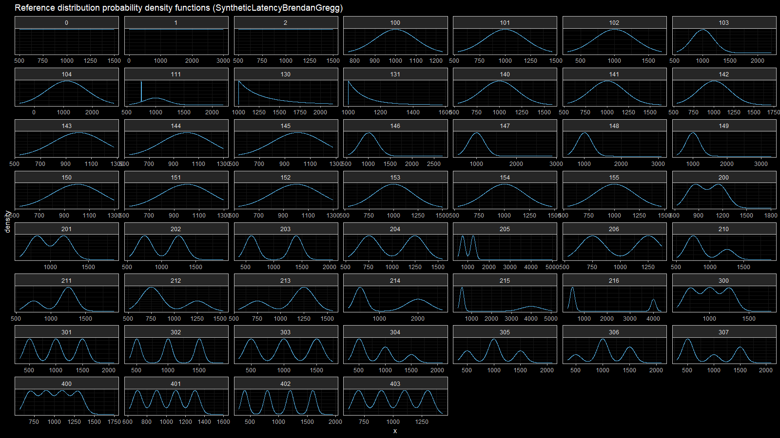
Here we can observe the same situation as in the previous section: HDQE is inefficient in the tail area of heavy-tailed distributions (with high outliers) and intermodal area of multimodal distributions.

Conclusion

In most simple cases, the Harrell-Davis quantile estimator is more efficient than the traditional one. However, it could be less efficient in areas closed to the low-density regions like tail areas of heavy-tailed distributions and intermodal areas of multimodal distributions.

References

• [Harrell1982]
  Harrell, F.E. and Davis, C.E., 1982. A new distribution-free quantile estimator. Biometrika, 69(3), pp.635-640.
  https://doi.org/10.2307/2335999
• [Hyndman1996]
  Hyndman, R. J. and Fan, Y. 1996. Sample quantiles in statistical packages, American Statistician 50, 361–365.
  https://doi.org/10.2307/2684934