Hodges-Lehmann Gaussian efficiency: location shift vs. shift of locations
Let us consider two samples $\mathbf{x} = (x_1, x_2, \ldots, x_n)$ and $\mathbf{y} = (y_1, y_2, \ldots, y_m)$. The one-sample Hodges-Lehmann EstimatorHodges-Lehman location estimator is defined as the median of the Walsh (pairwise) averages:
$$ \operatorname{HL}(\mathbf{x}) = \underset{1 \leq i \leq j \leq n}{\operatorname{median}} \left(\frac{x_i + x_j}{2} \right), \quad \operatorname{HL}(\mathbf{y}) = \underset{1 \leq i \leq j \leq m}{\operatorname{median}} \left(\frac{y_i + y_j}{2} \right). $$For these two samples, we can also define the shift between these two estimations:
$$ \Delta_{\operatorname{HL}}(\mathbf{x}, \mathbf{y}) = \operatorname{HL}(\mathbf{x}) - \operatorname{HL}(\mathbf{y}). $$The two-sample Hodges-Lehmann location shift estimator is defined as the median of pairwise differences:
$$ \operatorname{HL}(\mathbf{x}, \mathbf{y}) = \underset{1 \leq i \leq n,\,\, 1 \leq j \leq m}{\operatorname{median}} \left(x_i - y_j \right). $$Previously, I already compared the location shift estimator with the difference of median estimators (1, 2). In this post, I compare the difference between two location estimations and the shift estimations in terms of Gaussian efficiency. Before I started this study, I expected that $\operatorname{HL}$ should be more efficient than $\Delta_{\operatorname{HL}}$. Let us find out if my intuition is correct or not!
For the baseline, we consider the difference between the means:
$$ \Delta_{\operatorname{mean}}(\mathbf{x}, \mathbf{y}) = \operatorname{mean}(\mathbf{x}) - \operatorname{mean}(\mathbf{y}). $$The relative Gaussian efficiency of $\Delta_{\operatorname{HL}}$ and $\operatorname{HL}$ to $\Delta_{\operatorname{mean}}$ is defined as follows:
$$ \operatorname{eff}_{\mathcal{N}}(\Delta_{\operatorname{HL}}) = \frac{\mathbb{V}_{\mathcal{N}}[\Delta_{\operatorname{mean}}]}{\mathbb{V}_{\mathcal{N}}[\Delta_{\operatorname{HL}}]}, \quad \operatorname{eff}_{\mathcal{N}}(\operatorname{HL}) = \frac{\mathbb{V}_{\mathcal{N}}[\Delta_{\operatorname{mean}}]}{\mathbb{V}_{\mathcal{N}}[\operatorname{HL}]}. $$Numerical simulations
We conduct the following simulation:
- Enumerate the sample size $n$ from $3$ to $50$.
- For each $n$, generate $500\,000$ pairs of random samples from $\mathcal{N}(0, 1)$.
- For each pair of samples, estimate the shift between them using $\Delta_{\operatorname{HL}}$, $\operatorname{HL}$, and $\Delta_{\operatorname{mean}}$.
- Calculate the Gaussian efficiency of $\Delta_{\operatorname{HL}}$ and $\operatorname{HL}$ using the above equations.
Here are the results:
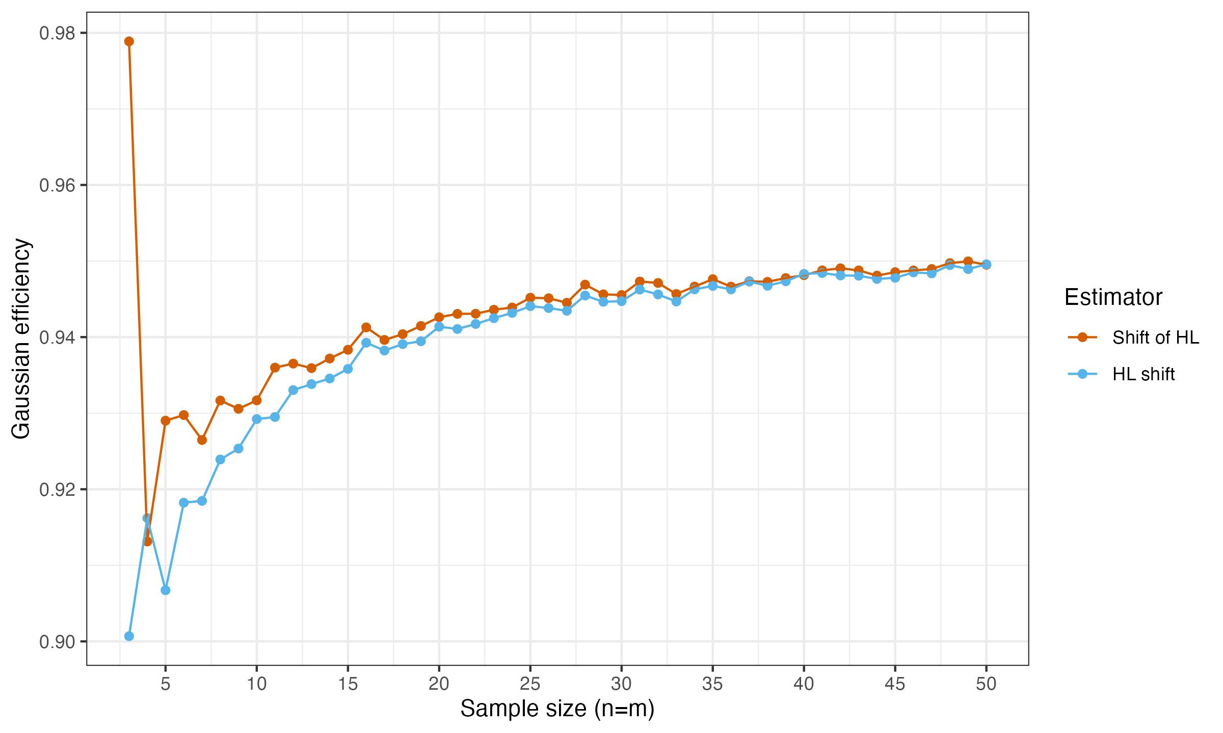
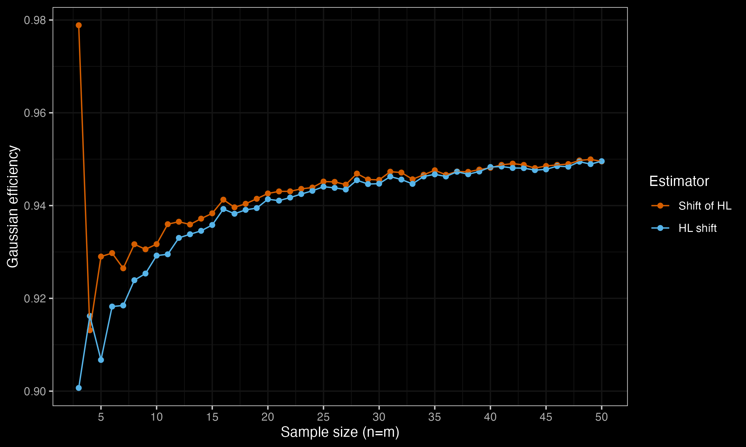
Surprisingly, but the shift of the Hodges-Lehmann location estimators $\Delta_{\operatorname{HL}}$ turned out to be more efficient under normality than Hodges-Lehmann location shift estimator $\operatorname{HL}$ (with the only exception of $n=m=4$). For $n,m \geq 15$, the difference is almost negligible, but it’s tangible for small sample sizes.
References
- [Hodges1963]
Hodges, J. L., and E. L. Lehmann. 1963. Estimates of location based on rank tests. The Annals of Mathematical Statistics 34 (2):598–611.
DOI:10.1214/aoms/1177704172