Joining modes of multimodal distributions
Multimodality of distributions is a severe issue in statistical analysis. Comparing two multimodal distributions is a tricky challenge. The degree of this challenge depends on the number of existing modes. Switching from unimodal models to multimodal ones can be a controversial decision, potentially causing more problems than solutions. Hence, if we dare to increase the complexity of the considering models, we should be sure that this is an essential necessity. Even when we confidently detect a truly multimodal distribution, a unimodal model could be an acceptable approximation if it is sufficiently close to the true distribution. The simplicity of a unimodal model may make it preferable, even if it is less accurate. Of course, the research goals should always be taken into account when the particular model choice is being made.
When we analyze samples of data and detect multimodality within them (e.g., using the lowland multimodality detector), we should always consider merging some modes. If the loss of accuracy during this transition is negligible in the context of the research goals, it is reasonable to simplify the model by joining the modes. For various kinds of situations, multiple decision-making strategies can be considered. Rather than using some of these strategies straightforwardly “as-is,” it is recommended to adjust them to each particular problem according to the existing limitations and business requirements. Let’s discuss a few use cases that demonstrate such strategies.
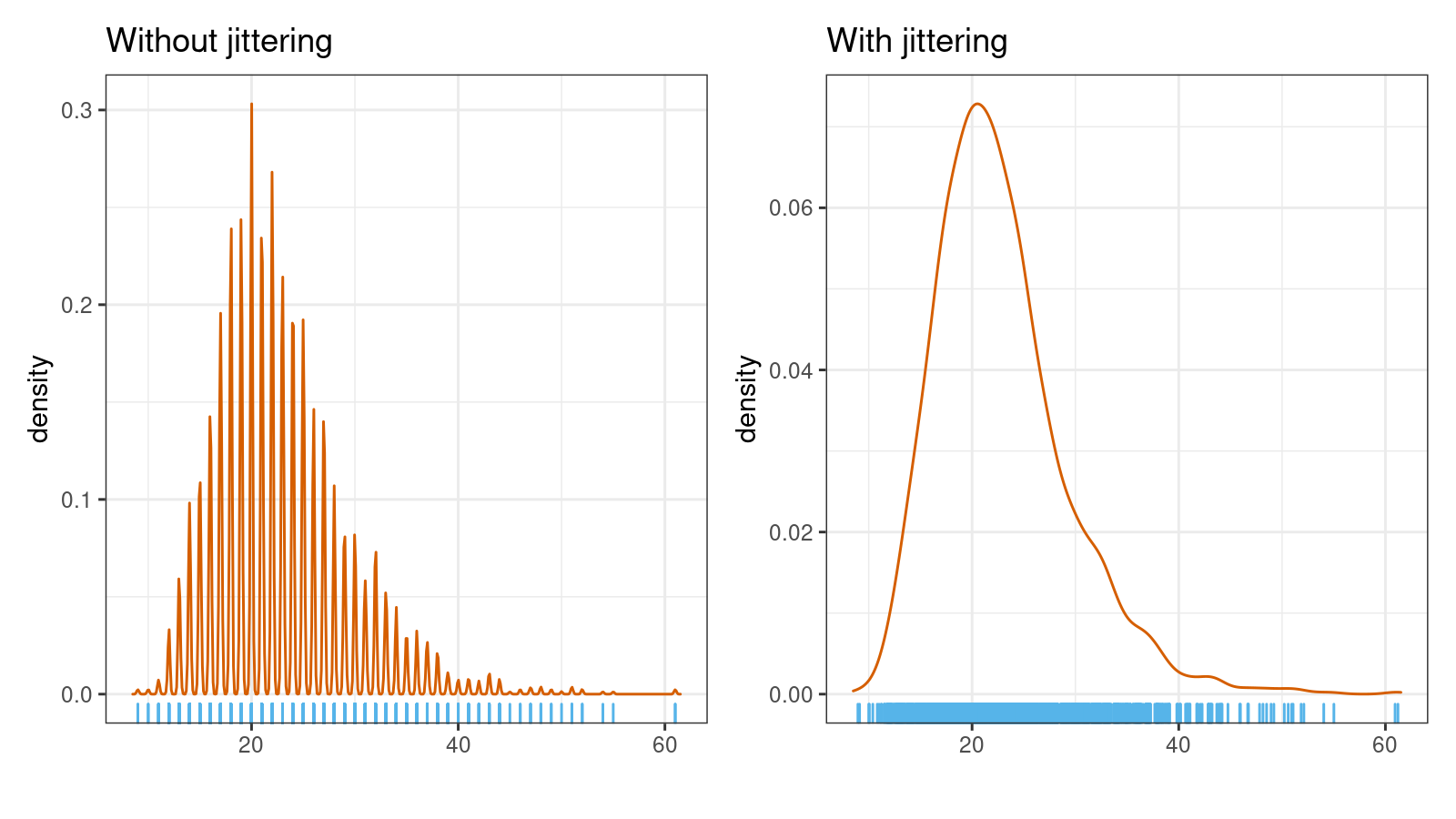
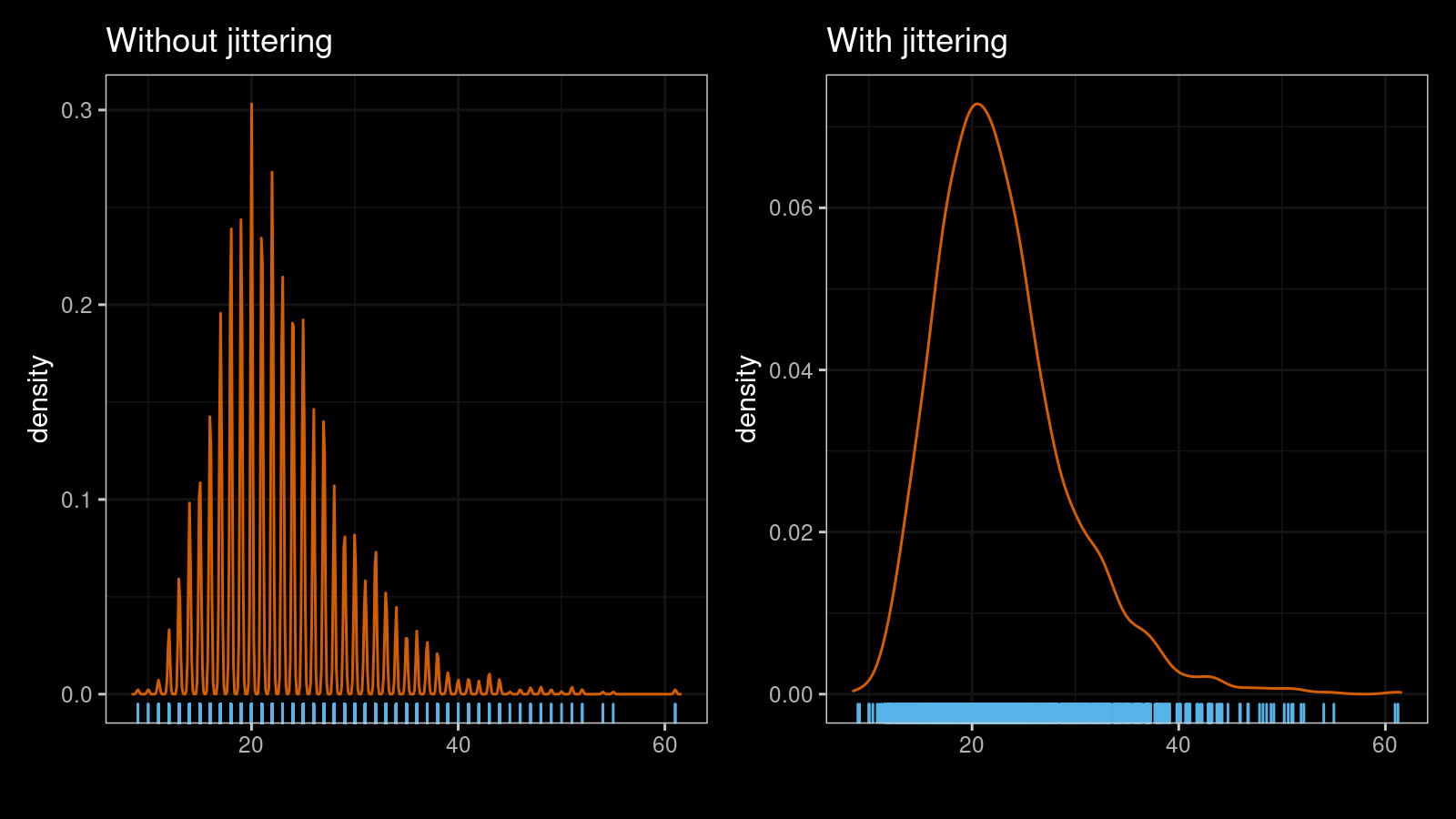
The first case appears when a continuous distribution becomes a discrete one because of the limited resolution of our measurement devices. In this case, if the given sample is sufficiently large, a multimodal detector can detect each discrete value as a separate mode. While such a model can be technically a correct one, it is not a reasonable option to consider for further analysis. The situation can be improved using jittering:
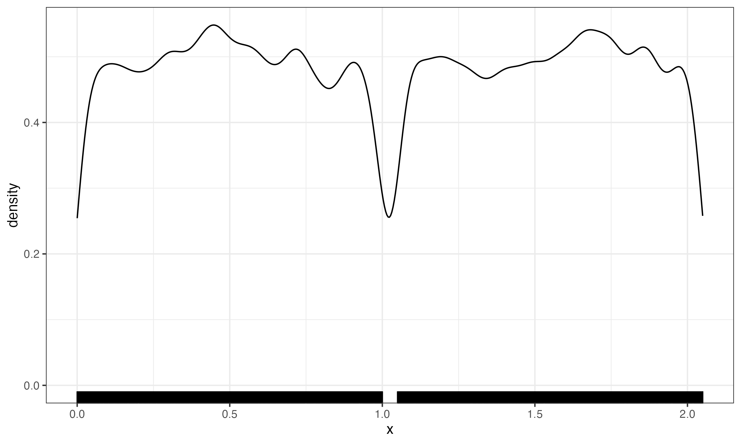
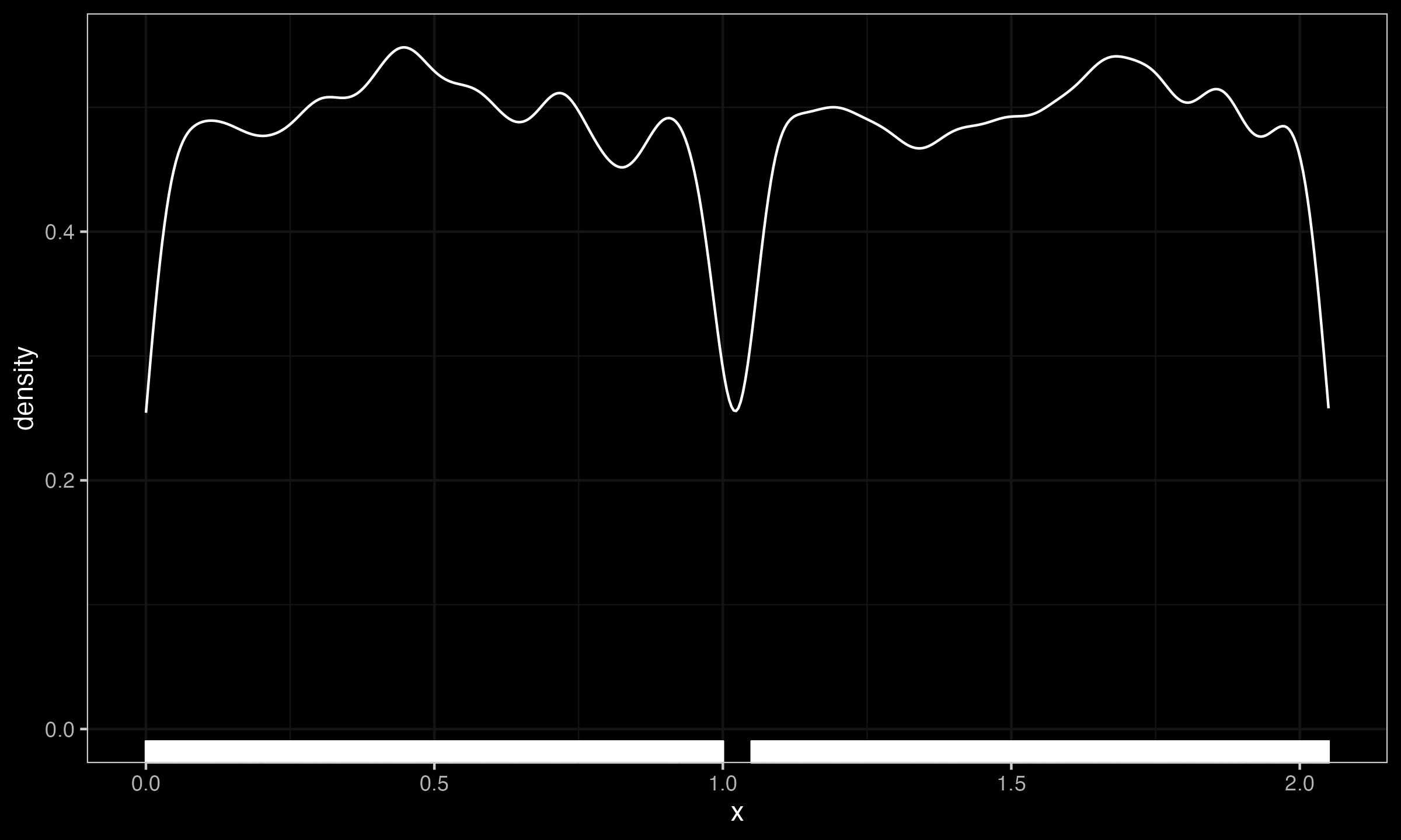
The second case appears when there is a small gap between two wide modes. For example, let us consider a mixture of two uniform distributions $\mathcal{U}(0, 1)$ and $\mathcal{U}(1.05, 2.05)$. While the gap between $1$ and $1.05$ can be easily detected on a huge sample size, for most applications, the whole distribution can be considered as $\mathcal{U}(0, 2.05)$ without noticeable loss of accuracy.
Note that each technique is designed for some specific cases: the jittering cannot be applied to the uniform mixture case, and the gap width analysis cannot be applied to discretized distributions. All of such techniques are just tools that you might use in some situations, but you should always verify their applicability.