Kernel density estimation and discrete values
Kernel density estimation (KDE) is a popular technique of data visualization.
Based on the given sample, it allows estimating the probability density function (PDF) of the underlying distribution.
Here is an example of KDE for x = {3.82, 4.61, 4.89, 4.91, 5.31, 5.6, 5.66, 7.00, 7.00, 7.00}
(normal kernel, Sheather & Jones bandwidth selector):
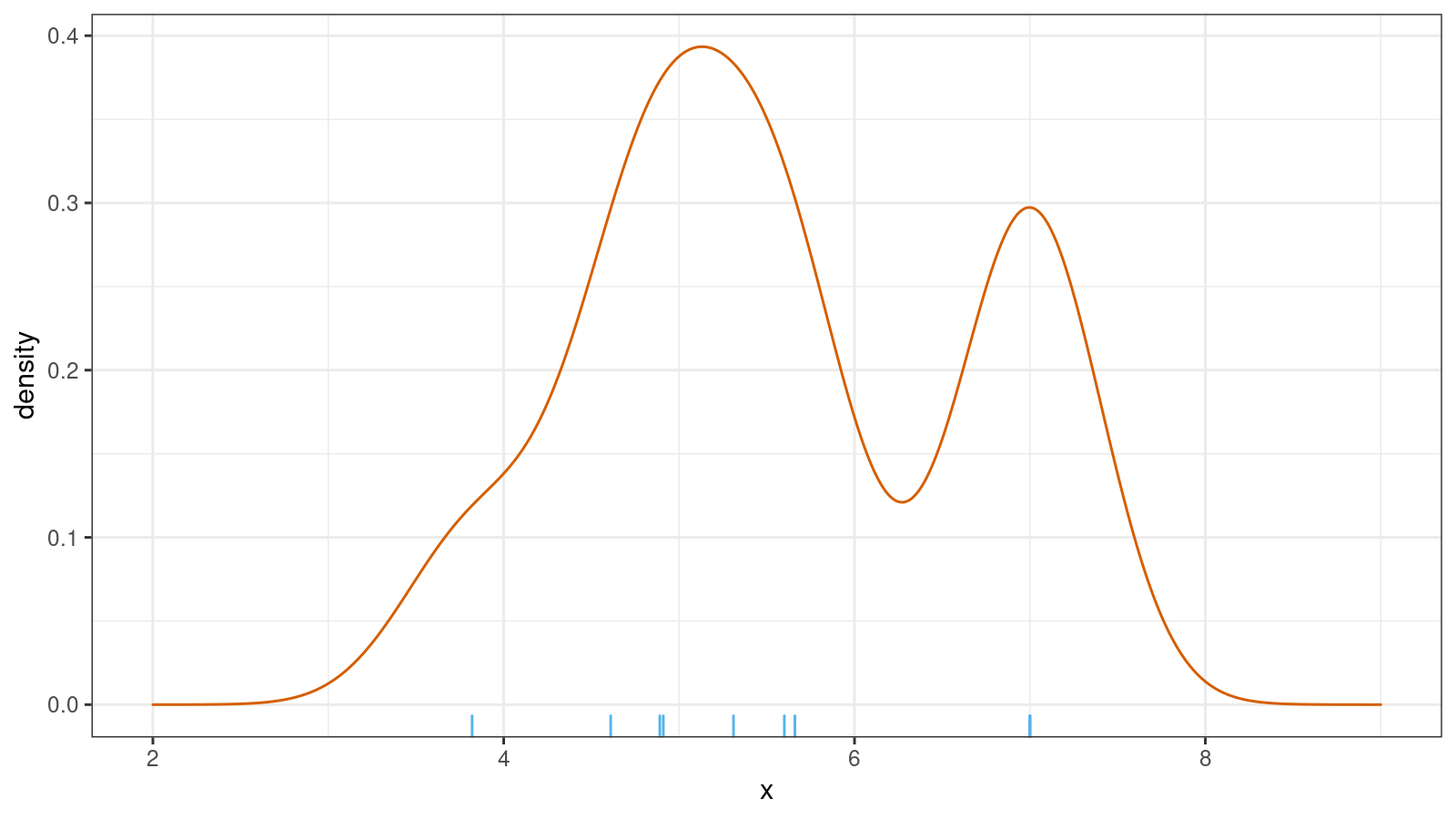
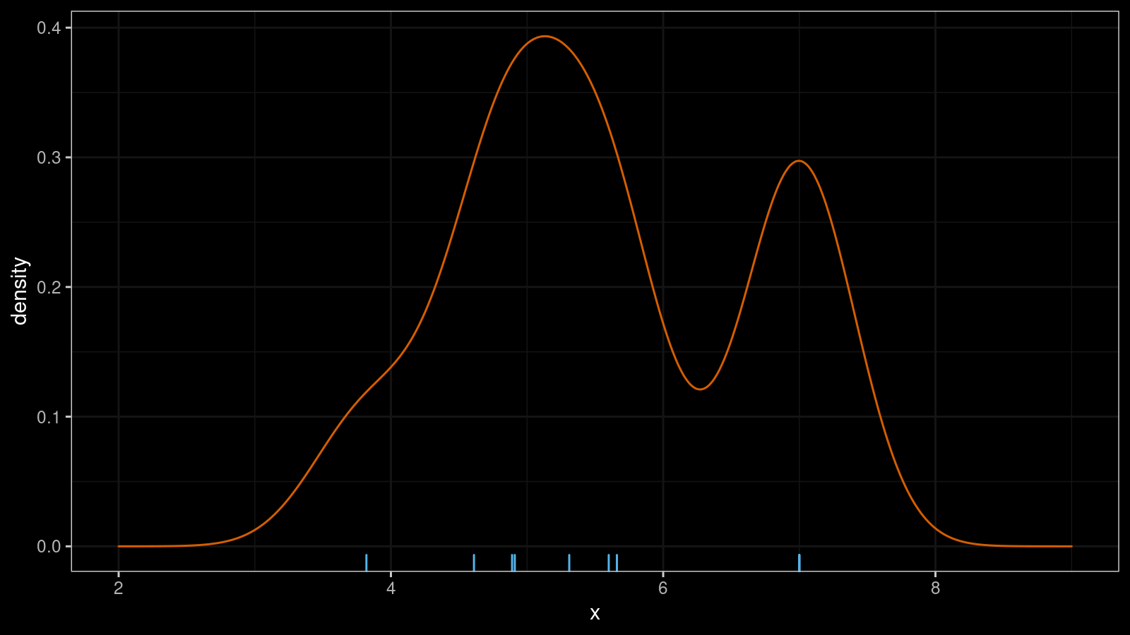
KDE is a simple and straightforward way to build a PDF, but it’s not always the best one. In addition to my concerns about bandwidth selection, continuous use of KDE creates an illusion that all distributions are smooth and continuous. In practice, it’s not always true.
In the above picture, the distribution looks pretty continuous.
However, the picture hides the fact that we have three 7.00 elements in the original sample.
With continuous distributions, the probability of getting tied observations (that have the same value) is almost zero.
If a sample contains ties, we are most likely working with
either a discrete distribution or a mixture of discrete and continuous distributions.
A KDE for such a sample may significantly differ from the actual PDF.
Thus, this technique may mislead us instead of providing insights about the true underlying distribution.
In this post, we discuss the usage of PDF and PMF with continuous and discrete distributions. Also, we look at examples of corrupted density estimation plots for distributions with discrete features.
PDF and continuous distributions
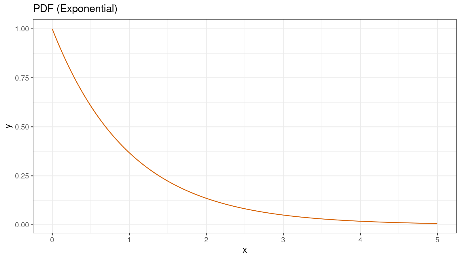
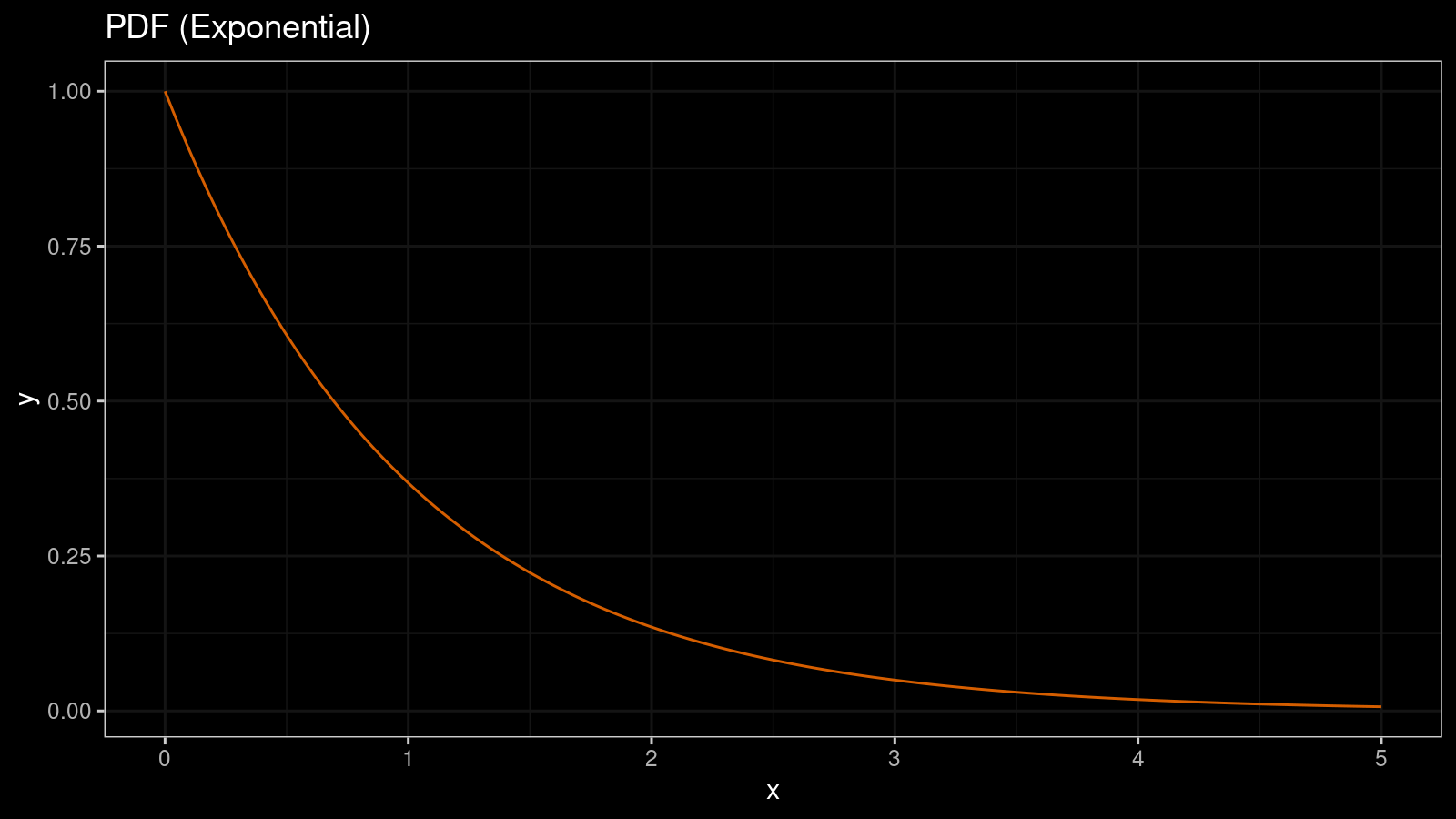
One of the simplest ways to visualize the shape of a distribution is to draw its probability density function (PDF). Typically, such function is denoted as $f(x)$. For example, for exponential distribution, $f(x) = \lambda e^{-\lambda x}$. Here is how it looks like:
If we want to know the probability of falling a random variable $X$ inside an interval $[a;b]$, we should calculate the integral of $f(x)$ on this interval:
$$ P[a \leq X \leq b] = \int_a^b f(x) dx. $$In the case of absolutely continuous distributions with finite values of $f(x)$, the probability of getting the given constant $a$ as a realization of random variable $X$ is zero:
$$ P[X = a] = \int_a^a f(x) dx = 0. $$PMF and discrete distributions
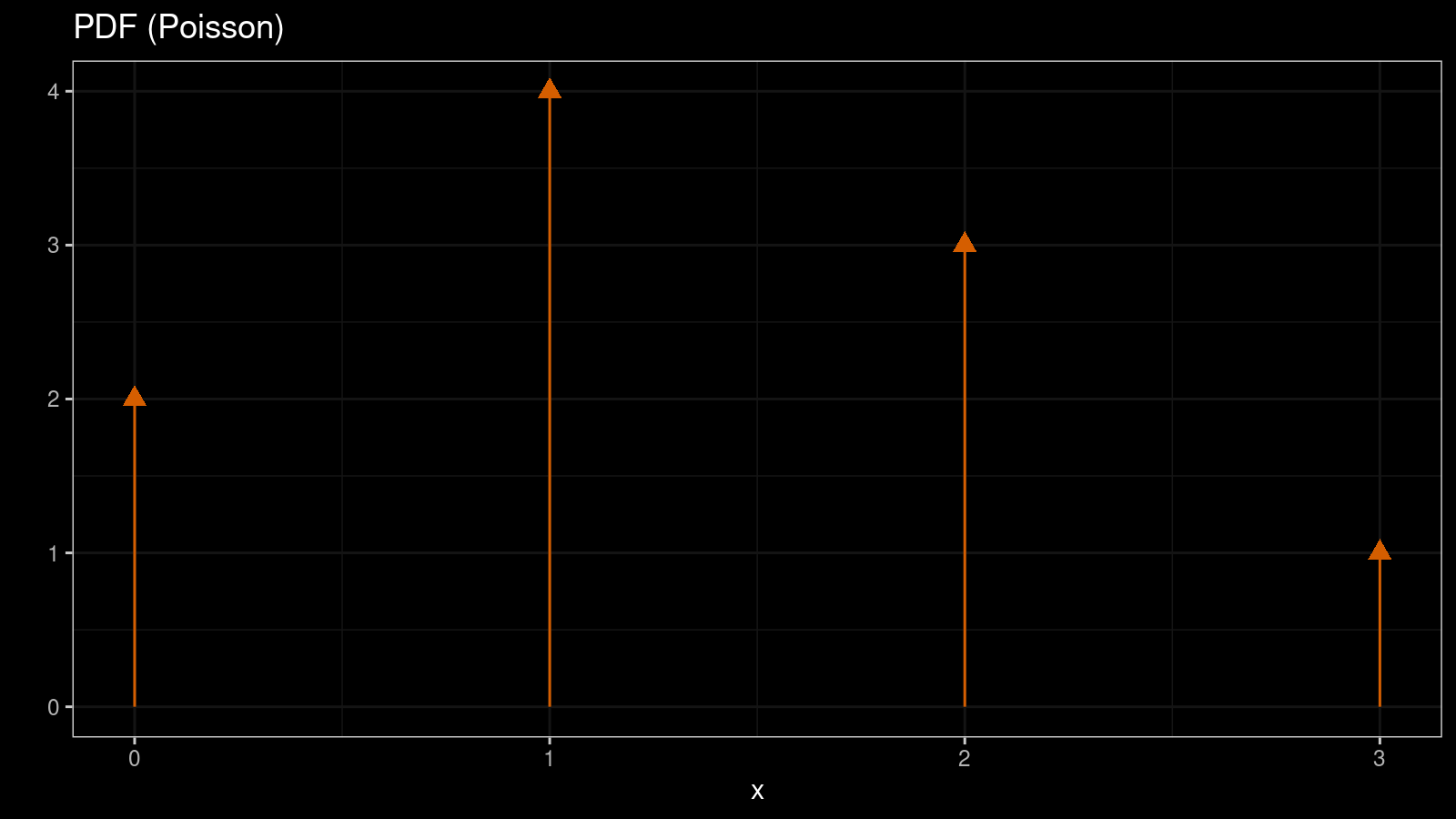
In some cases, we have to work with discrete distributions that allow only discrete values from a countable set of numbers (e.g., 1, 2, 3, etc.). In this case, we typically use probability mass function (PMF) instead of PDF. PMF gives us the probability of getting a specific value. For example, here is PMF for the Poisson distribution:
$$ f(k) = \frac{\lambda^k e^{-\lambda}}{k!} \quad \Big( k \in \mathcal{N}_0 \Big) $$The easiest way to visualize a PMF is a histogram. Here is the corresponding histogram for the Poisson distribution:
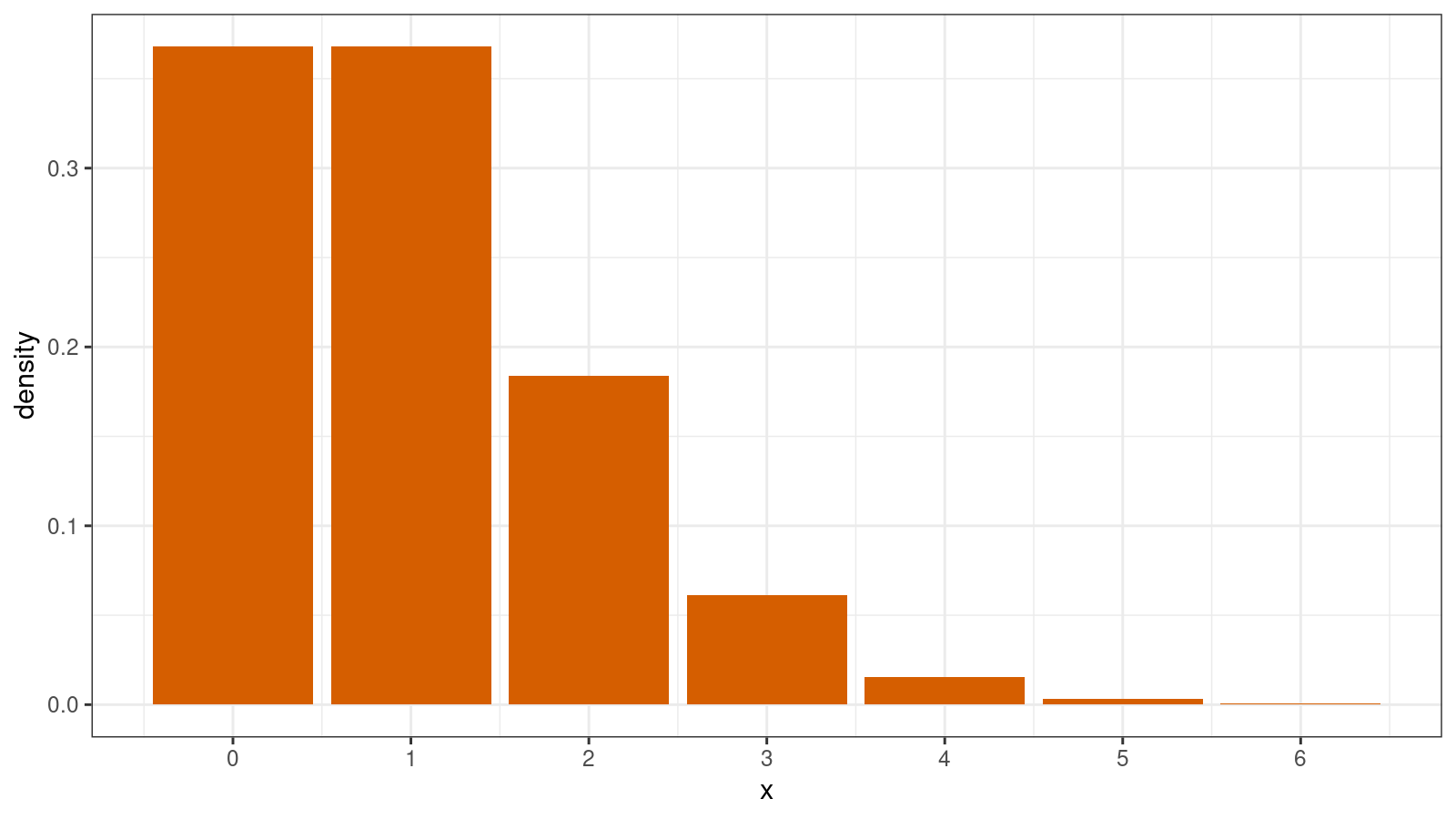
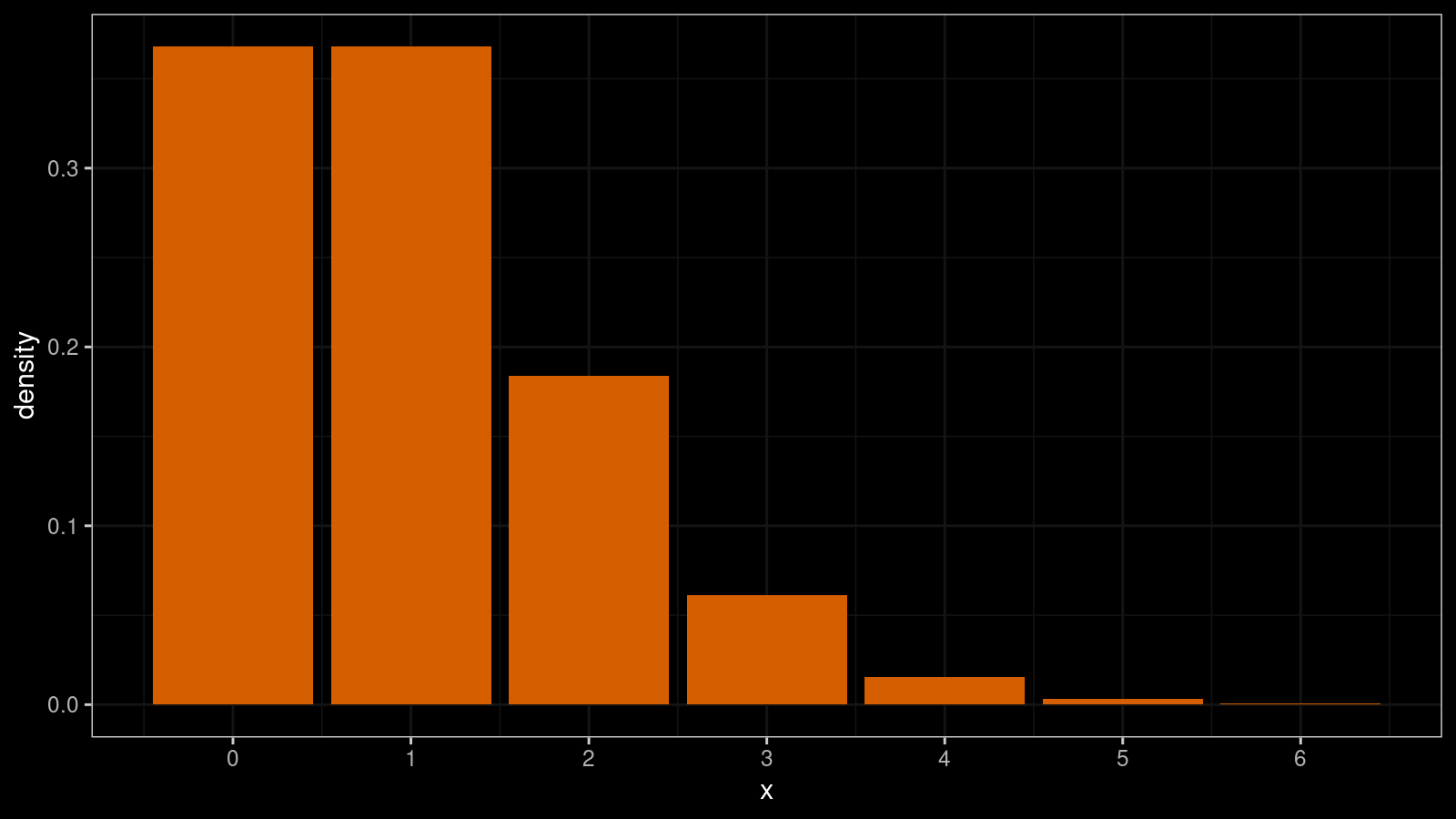
In the case of a discrete distribution, we typically don’t have problems with the bin width and the offset. In the simplest case, we can just display a bar per each discrete value. However, if the discretization step is too small, we will have to group values to get a meaningful image.
KDE and discrete distributions
Treating discrete distributions as continuous distributions may lead to some undesired effects.
Let’s build a KDE1 for a random sample from the Poisson distribution (x = {2, 3, 0, 2, 1, 1, 2, 0, 1, 1}):
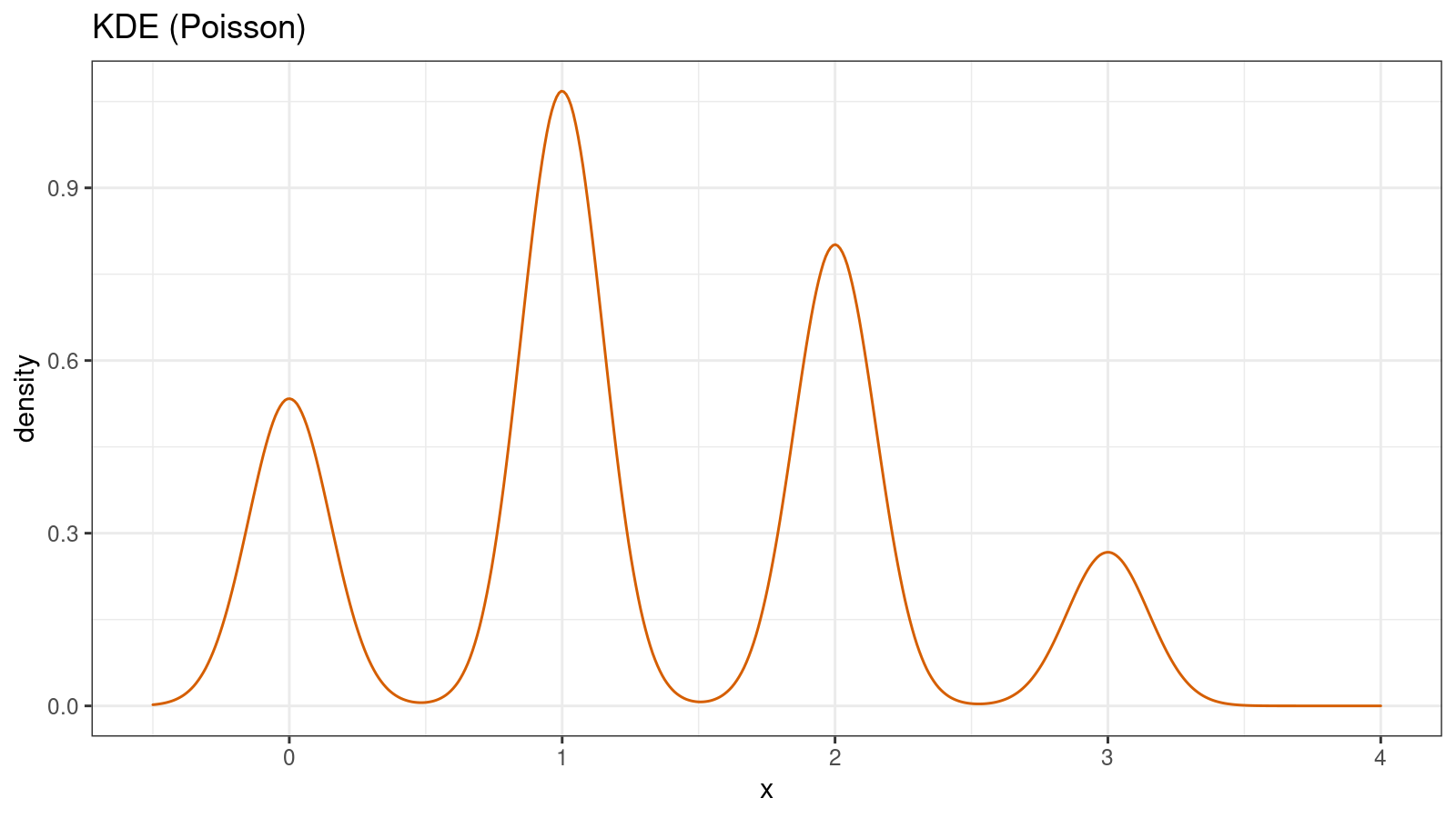
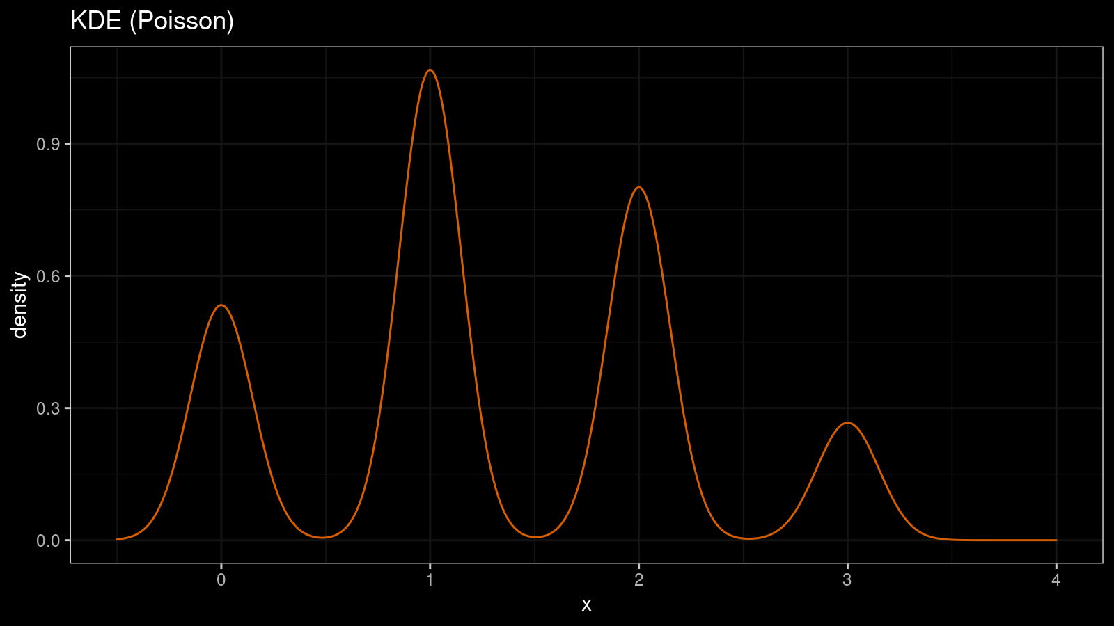
Such visualization creates a false feeling of a continuous distribution. We could think that this distribution is multimodal while it’s actually unimodal. We could think that there is a high probability of real numbers while
PDF and discrete distributions
Strictly speaking, PDF is not defined for discrete distributions. However, we could try to define it using the Dirac delta function:
$$ \delta(x) = \begin{cases} +\infty, & x = 0 \\ 0, & x \ne 0 \end{cases}, $$$$ \int_{-\infty}^\infty \delta(x) \, dx = 1. $$For example, for the Poisson distribution, the PDF can be defined as follows:
$$ f(x) = \sum_{i=0}^\infty \frac{\lambda^x e^{-\lambda}}{x!} \cdot \delta(x - i) $$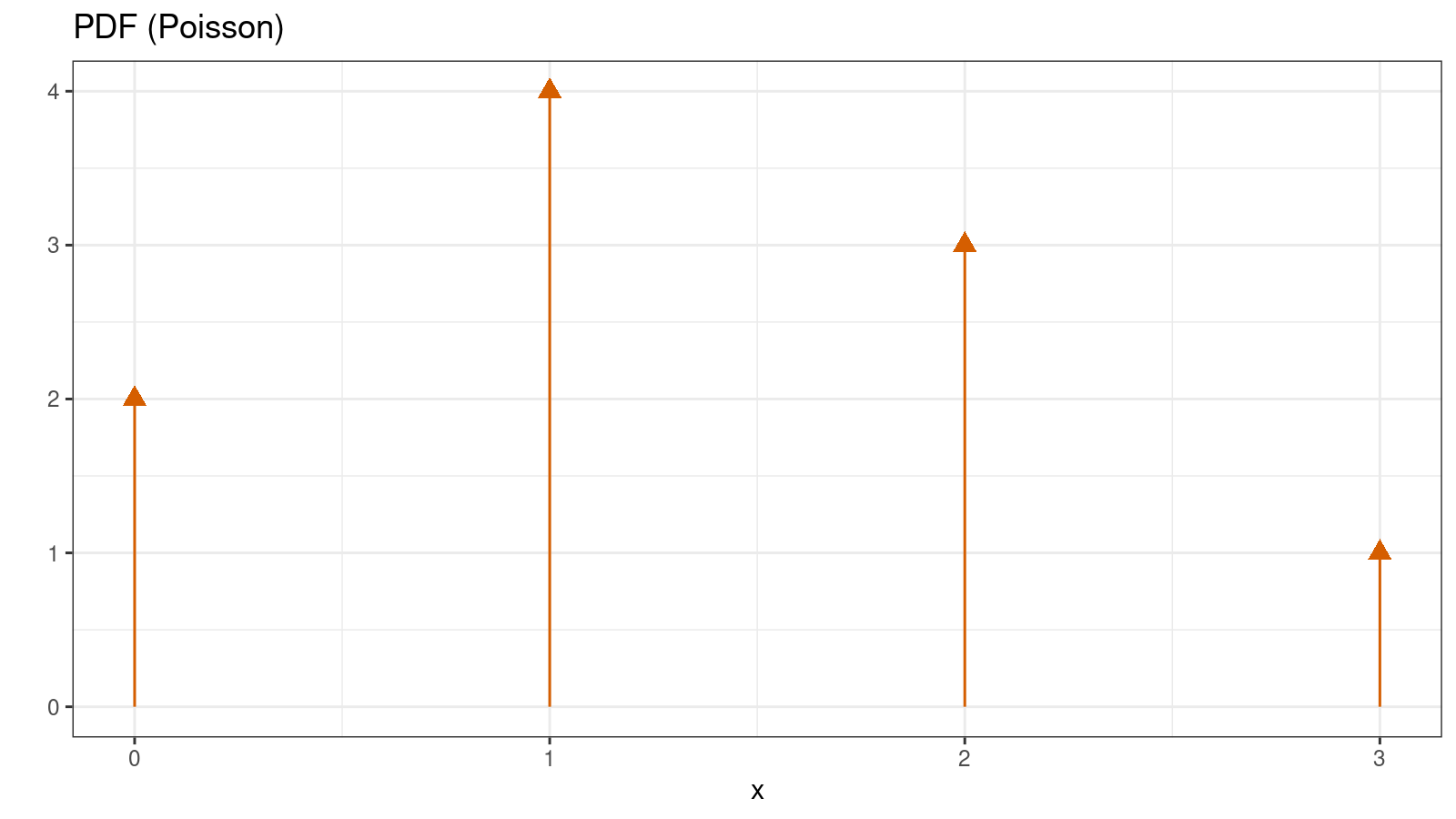
Sometimes, such PDF is referenced as generalized PDF. It allows working with continuous and discrete distributions the same way.
PDF and mixed distributions
We can also consider a mixture of a discrete distribution and a continuous distribution. One of the most famous examples of mixed discrete/continuous distributions is the rectified Gaussian distribution. This distribution can be obtained from the Gaussian distribution by replacing all negative values with zeros. Here is the PDF of the rectified Gaussian distribution:
$$ f(x) = \Phi\Big(-\frac{\mu}{\sigma}\Big)\delta(x)+ \frac{1}{\sqrt{2\pi\sigma^2}}\; e^{ -\frac{(x-\mu)^2}{2\sigma^2}}\textrm{U}(x) $$where $\Phi(x)$ is the CDF of the standard normal distribution, $\delta(x)$ is the Dirac delta function, $\textrm{U}(x)$ is the unit step function.
And here are the PDF plots of the standard Gaussian, rectified Gaussian, and truncated Gaussian distributions:
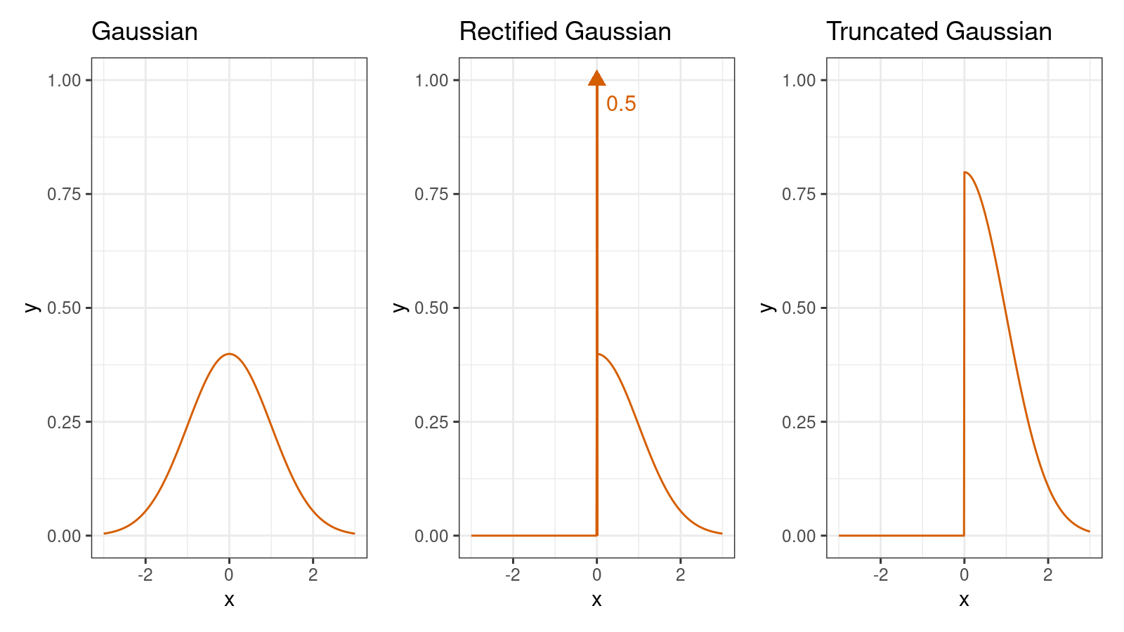
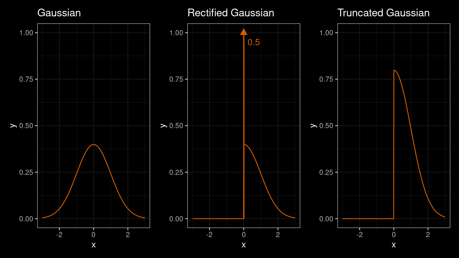
The most important thing about the standard rectified Gaussian distribution is that
we get the value 0 with the probability 0.5.
It’s hard to highlight this fact on the PDF plot, but we could try to do it using the Dirac delta function.
Real-life distributions: from continuous to discrete
There are many real-life distributions that we treat as continuous.
However, in some cases, these distributions may accidentally become discrete.
A typical source of discretization is a limited resolution of the used measuring tool.
Let’s say we have a sample x = {4.188, 4.216, 4.568, 5.321, 5.432, 5.655, 6.444}.
Is it discrete or continuous?
At first sight, it may look like a sample from a continuous distribution.
However, we can also notice that all values have exactly 3 digits after the decimal point.
If it’s the actual resolution of our measurement tool (the resolution is insufficient to get the fourth digit),
we can treat this distribution as a discrete one.
Indeed, it’s impossible to obtain any measurements between 0.001 and 0.002 with such a resolution.
It’s important because when the number of observations is high,
we can easily get the undersmoothing problem.
Here is another example of KDE1 that illustrates the problem:

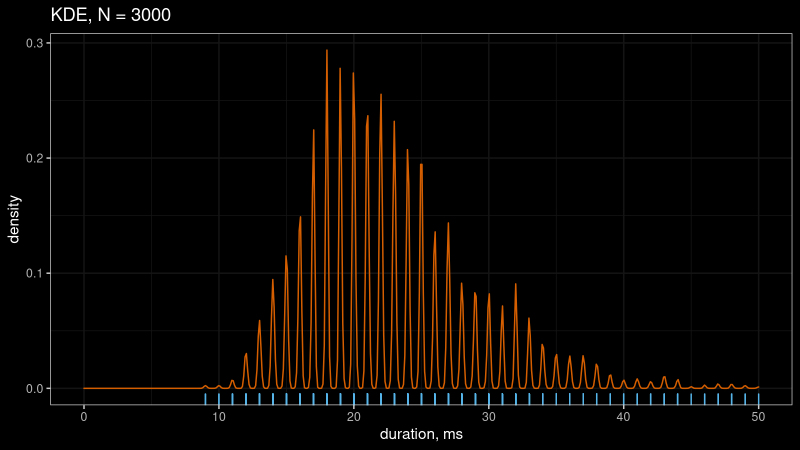
This estimation was formed based on a sample (N=3000) of short durations rounded to milliseconds. Rounding leads to artificial discretization, which leads to undersmoothing. As a result, we have a serrated pattern instead of a nice-looking smooth approximation.
Real-life distribution: from continuous to mixed
Another source of problems is boundary values. For example, if a distribution consists of non-negative numbers, it’s a typical situation when some of the measurements are equal to zero. If we have an upper limit for measurements, we could expect that some values are equal to this limit.
Here is another KDE1 based on a sample from the rectified Gaussian distribution:
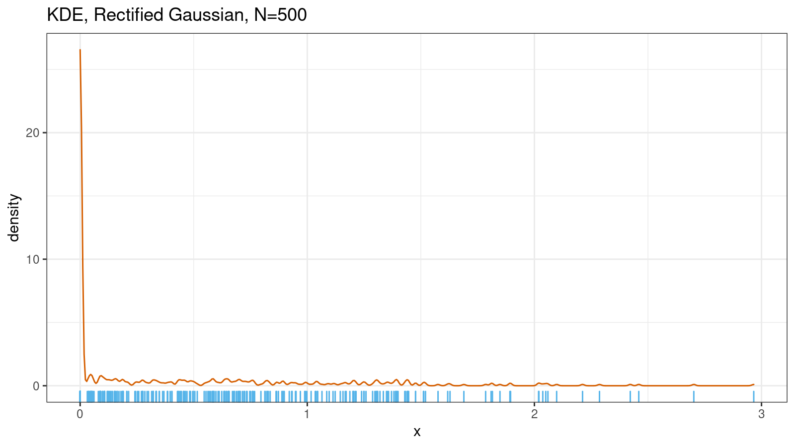

The plot focuses our attention on the fact that most of the sample values are around zero, but it hides the shape of the distribution in the non-zero region. Also, it hides the ratio of zero and non-zero values. In fact, only a half of the values are zeros; another half has the shape of the truncated gaussian distribution.
Conclusion
There are many real-life distributions that we consider continuous. Even when they are truly continuous, the collected data may belong to a discrete distribution or mixed discrete/continuous distributions. If a sample contains tied values, the distribution is most probably has discrete features. In this case, you should be careful with density estimation. Some common ways to estimate density, like kernel density estimation, may mislead you using corrupted visualizations.