Using Kish's effective sample size with weighted quantiles

In my previous posts, I described how to calculate weighted quantiles and their confidence intervals using the Harrell-Davis quantile estimator. This powerful technique allows applying quantile exponential smoothing and dispersion exponential smoothing for time series in order to get its moving properties.

When we work with weighted samples, we need a way to calculate the effective samples size. Previously, I used the sum of all weights normalized by the maximum weight. In most cases, it worked OK.

Recently, Ben Jann pointed out that it would be better to use the Kish’s formula to calculate the effective sample size. In this post, you find the formula and a few numerical simulations that illustrate the actual impact of the underlying sample size formula.

Let’s say we have a sample $x = \{ x_1, x_2, \ldots, x_n \}$ with a vector of corresponding weights $w = \{ w_1, w_2, \ldots, w_n \}$. In the non-weighted case (when all weights $w_i$ are equal), we can safely use the sample size $n$ in all equations that required the sample size. However, in the weighted case (when we have different values in $w$), we should perform some adjustments and calculate the effective sample size. Initially, I used the sum of all weights normalized by the maximum element:

In kish1965, there is a better way to estimate the effective sample size:

Let’s compare both approaches on a few data sets. First, let’s check the time series with two change points from the original post:

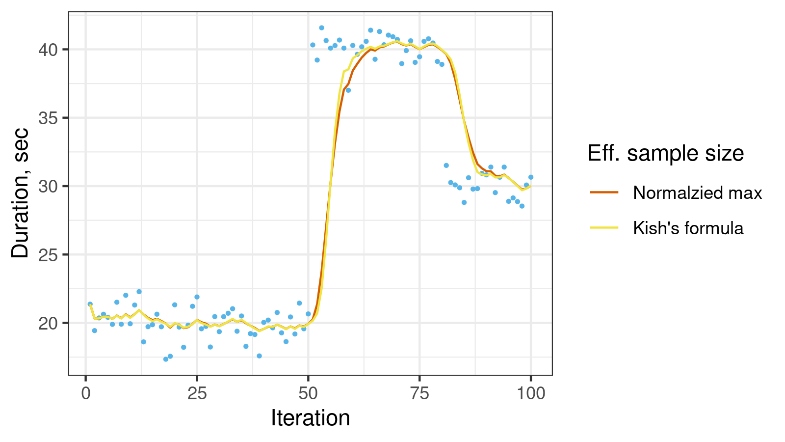
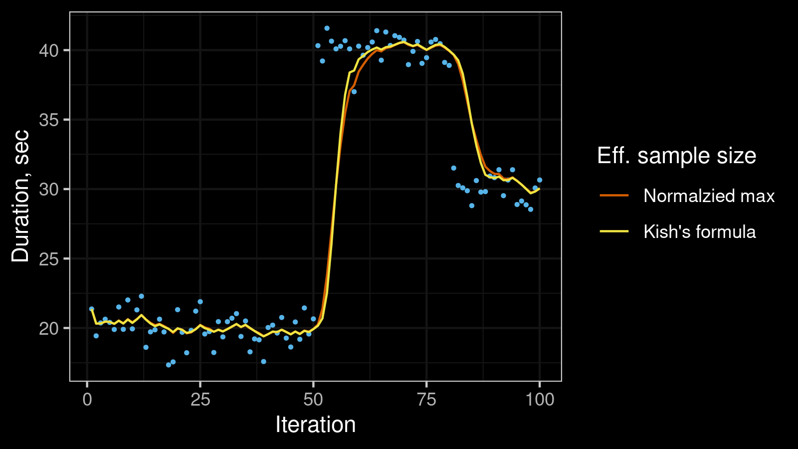
Here we estimate the moving median using exponential smoothing with lifetime = 5. As we can see, the Kish’s formula gives a shorter “retraining interval” after each change point.

Now let’s try another time series from the quantile exponential smoothing post with (monotonically increasing sine wave pattern with high outliers):

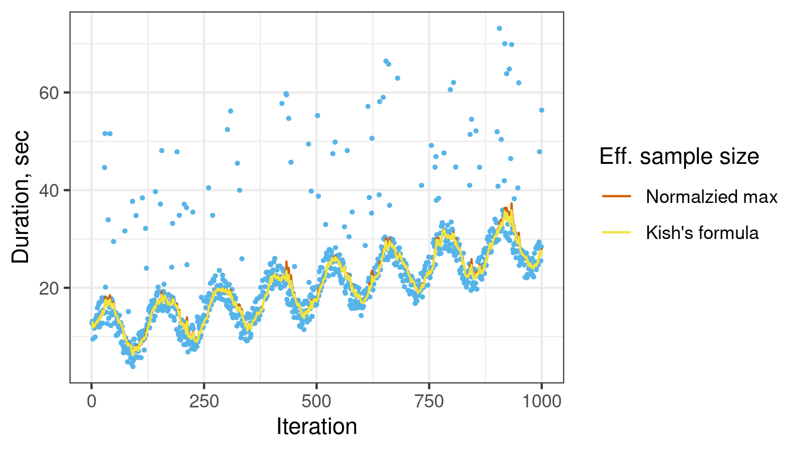
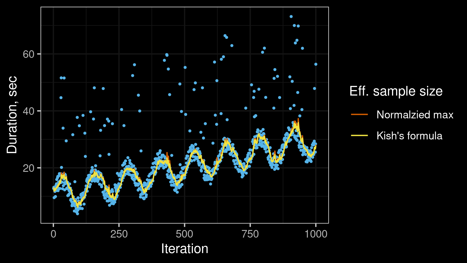
Here we can notice that the Kish’s formula is more resistant to outliers (it gives a smoother line with a fewer number of sharp peaks).

I have performed a series of additional experiments, and all of them have shown that the Kish’s formula provides better results. Of course, it worth to carefully measure the statistical efficiency of both options. However, based on the first impression, the Kish’s effective sample size is my new approach of choice. Thanks again to Ben Jann for the valuable hint!

References

• [Kish1965]
  Kish, Leslie. Survey sampling. Chichester., 1965.
  https://doi.org/10.1002/bimj.19680100122