Quantile estimators based on k order statistics, Part 2: Extending Hyndman-Fan equations

In the previous post, I described the idea of using quantile estimators based on k order statistics. Potentially, such estimators could be more robust than estimators based on all samples elements (like Harrell-Davis, Sfakianakis-Verginis, or Navruz-Özdemir) and more statistically efficient than traditional quantile estimators (based on 1 or 2 order statistics). Moreover, we should be able to control this trade-off based on the business requirements (e.g., setting the desired breakdown point).

The only challenging thing here is choosing the weight function that aggregates k order statistics to a single quantile estimation. We are going to try several options, perform Monte-Carlo simulations for each of them, and compare the results. A reasonable starting point is an extension of the traditional quantile estimators. In this post, we are going to extend the Hyndman-Fan Type 7 quantile estimator (nowadays, it’s one of the most popular estimators). It estimates quantiles as a linear interpolation of two subsequent order statistics. We are going to make some modifications, so a new version is going to be based on k order statistics.

Spoiler: this approach doesn’t seem like an optimal one. I’m pretty disappointed with its statistical efficiency on samples from light-tailed distributions. So, what’s the point of writing a blog post about an inefficient approach? Because of the following reasons:

1. I believe it’s crucial to share negative results. Sometimes, knowledge about approaches that don’t work could be more important than knowledge about more effective techniques. Negative results give you a broader view of the problem and protect you from wasting your time on potential promising (but not so useful) ideas.
2. Negative results improve research completeness. When we present an approach, it’s essential to not only show why it solves problems well, but also why it solves problems better than other similar approaches.
3. While I wouldn’t recommend my extension of the Hyndman-Fan Type 7 quantile estimator to the k order statistics case as the default quantile estimator, there are some specific cases where it could be useful. For example, if we estimate the median based on small samples from a symmetric light-tailed distribution, it could outperform not only the original version but also the Harrell-Davis quantile estimator. The “negativity” of the negative results always exists in a specific context. So, there may be cases when negative results for the general case transform to positive results for a particular niche problem.
4. Finally, it’s my personal blog, so I have the freedom to write on any topic I like. My blog posts are not publications to scientific journals (which typically don’t welcome negative results), but rather research notes about conducted experiments. It’s important for me to keep records of all the experiments I perform regardless of the usefulness of the results.

So, let’s briefly look at the results of this not-so-useful approach.

All posts from this series:

• Quantile estimators based on k order statistics, Part 1: Motivation (August 3, 2021)
• Quantile estimators based on k order statistics, Part 2: Extending Hyndman-Fan equations (August 10, 2021)
• Quantile estimators based on k order statistics, Part 3: Playing with the Beta function (August 17, 2021)
• Quantile estimators based on k order statistics, Part 4: Adopting trimmed Harrell-Davis quantile estimator (August 24, 2021)
• Quantile estimators based on k order statistics, Part 5: Improving trimmed Harrell-Davis quantile estimator (August 31, 2021)
• Quantile estimators based on k order statistics, Part 6: Continuous trimmed Harrell-Davis quantile estimator (September 7, 2021)
• Quantile estimators based on k order statistics, Part 7: Optimal threshold for the trimmed Harrell-Davis quantile estimator (September 14, 2021)
• Quantile estimators based on k order statistics, Part 8: Winsorized Harrell-Davis quantile estimator (September 21, 2021)

The approach

To make the generalization of the traditional quantile estimators, I’m going to continue developing the idea that I described in the post about weighted quantile estimators. Let’s say we have a sorted sample $x = \{ x_1, x_2, \ldots, x_n \}$ and we want to estimate the $p^\textrm{th}$ quantile $q_p$. For the original Hyndman-Fan Type 7 quantile estimators, we should set $h = (n-1)p+1$ and use the following formula:

$$ q_p = x_{\lfloor h \rfloor} + (h - \lfloor h \rfloor) (x_{\lfloor h \rfloor + 1} - x_{\lfloor h \rfloor}). $$

In order to build a generalization, we could express the $p^\textrm{th}$ quantile as a weighted sum of all order statistics:

$$ \begin{gather*} q_p = \sum_{i=1}^{n} W_{i} \cdot x_i,\\ W_{i} = F(r_i) - F(l_i),\\ l_i = (i - 1) / n, \quad r_i = i / n. \end{gather*} $$

where $F$ is a CDF function of a distribution that defines the element weights. In the case of the Hyndman-Fan Type 7 quantile estimator, this distribution could be defined as follows:

$$ F_7(u) = \left\{ \begin{array}{lcrcllr} 0 & \textrm{for} & & & u & < & (h-1)/n, \\ un-h+1 & \textrm{for} & (h-1)/n & \leq & u & \leq & h/n, \\ 1 & \textrm{for} & h/n & < & u. & & \end{array} \right. $$

The corresponding PDF (let’s call it $f_7$) looks simpler:

$$ f_7(u) = F'_7(u) = \left\{ \begin{array}{lcrcllr} 0 & \textrm{for} & & & u & < & (h-1)/n, \\ n & \textrm{for} & (h-1)/n & \leq & u & \leq & h/n, \\ 0 & \textrm{for} & h/n & < & u. & & \end{array} \right. $$

For example, if $n=5$, $p=0.25$, we have $h=2.4$ and the following PDF/CDF plots:

As we can see, the width of the non-zero-PDF-window is $1/h$ which covers at most two order statistics. To make the k order statistics generalization, we could just extend the window size! So, the updated PDF/CDF equations could be defined as follows:

$$ F_{7:k}(u) = \left\{ \begin{array}{lcrcllr} 0 & \textrm{for} & & & u & < & L_k, \\ (u-L_k)/(R_k-L_k) & \textrm{for} & L_k & \leq & u & \leq & R_k, \\ 1 & \textrm{for} & R_k & < & u. & & \end{array} \right. $$ $$ f_{7:k}(u) = F'_{7:k}(u) = \left\{ \begin{array}{lcrcllr} 0 & \textrm{for} & & & u & < & L_k, \\ 1/(R_k-L_k) & \textrm{for} & L_k & \leq & u & \leq & R_k, \\ 0 & \textrm{for} & R_k & < & u. & & \end{array} \right. $$

We already know values of $L_k$ and $R_k$ for $k=2$:

$$ L_2 = (h-1)/n, \quad R_2 = h/n. $$

We want $L_k$, $R_k$ to satisfy the following conditions:

$$ R_k-L_k = (k-1)/n, \quad L_k(h=1) = 0, \quad R_k(h=n) = 1. $$

Thus, we have (assuming $k - 1 \leq n$):

$$ L_k = (h - 1) / (n - 1) \cdot (n - (k - 1)) / n, \quad R_k = L_k + (k-1)/n. $$

That’s all! It’s time to verify these equations in numerical simulations!

Numerical Simulations

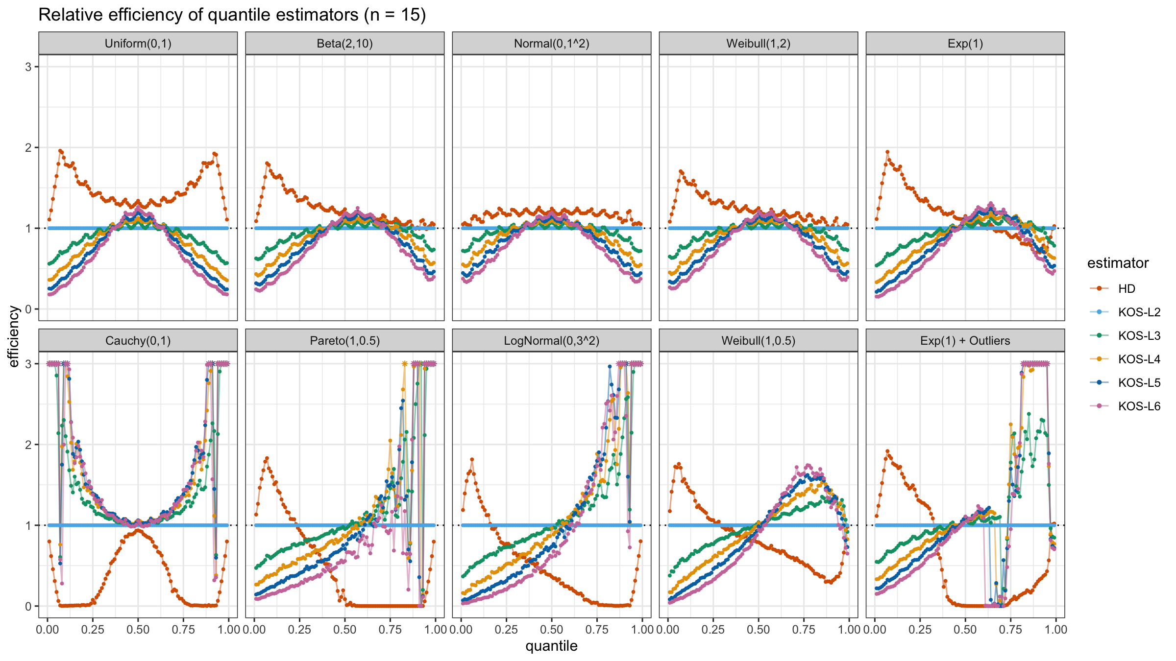
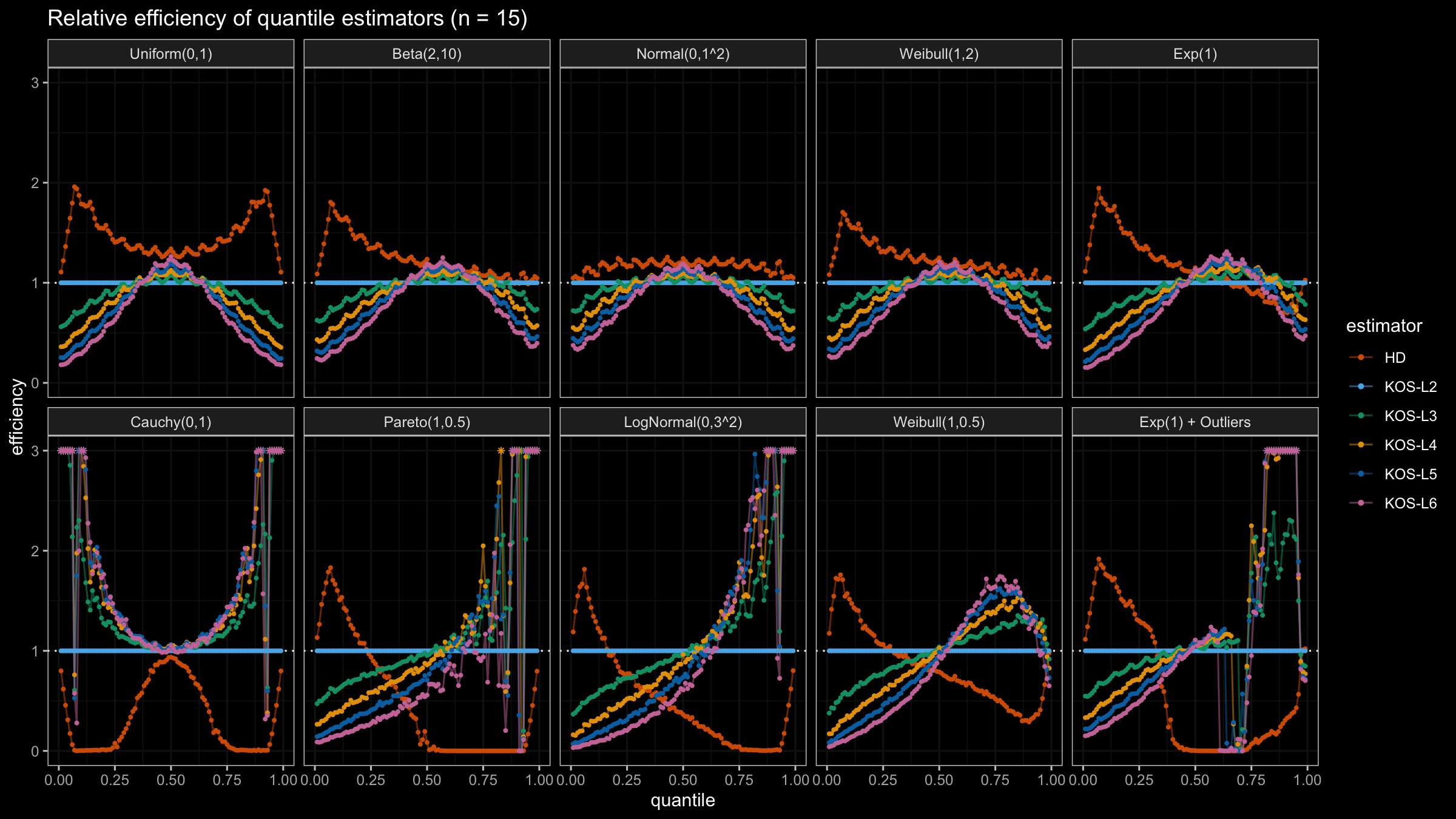
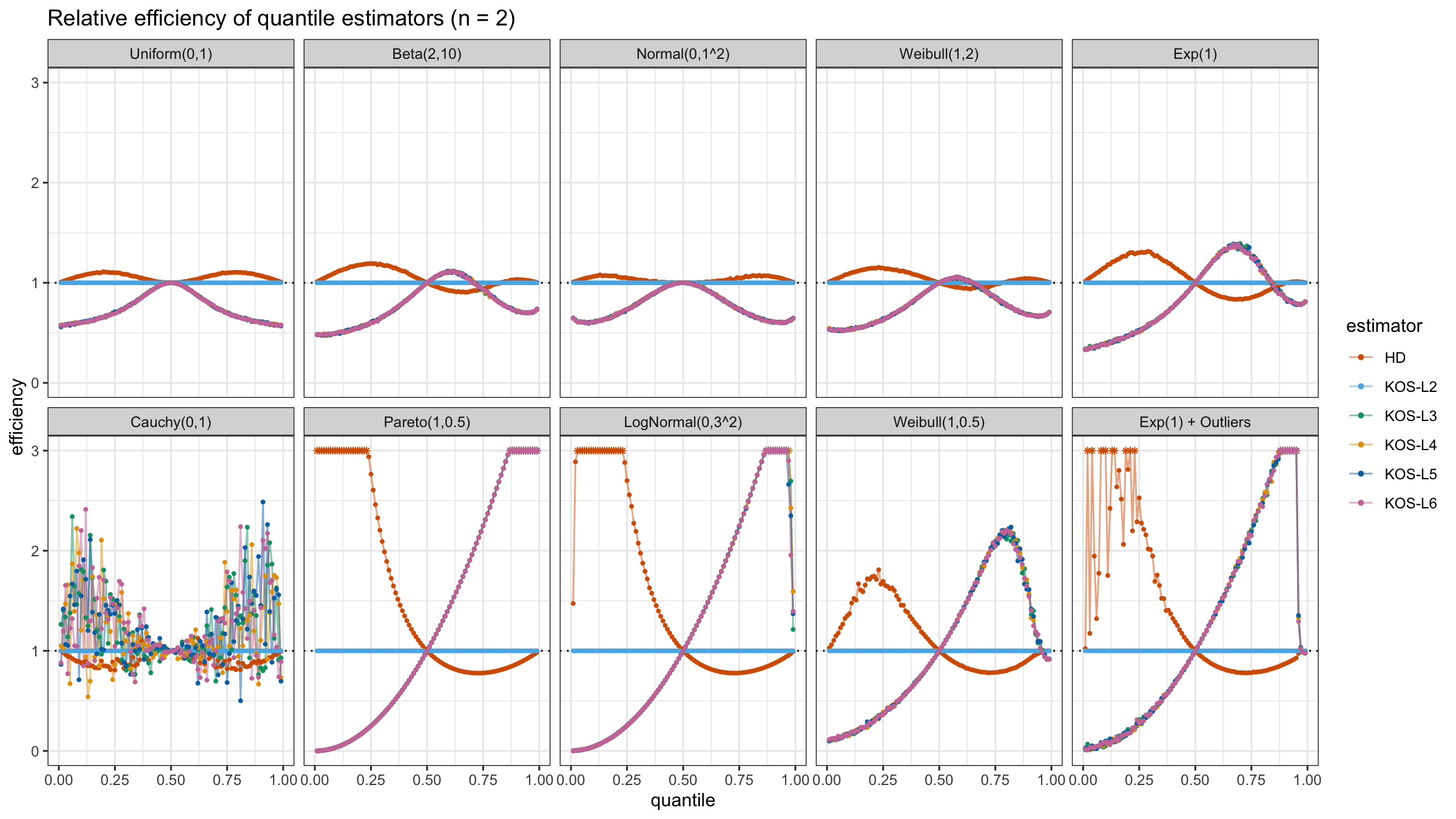
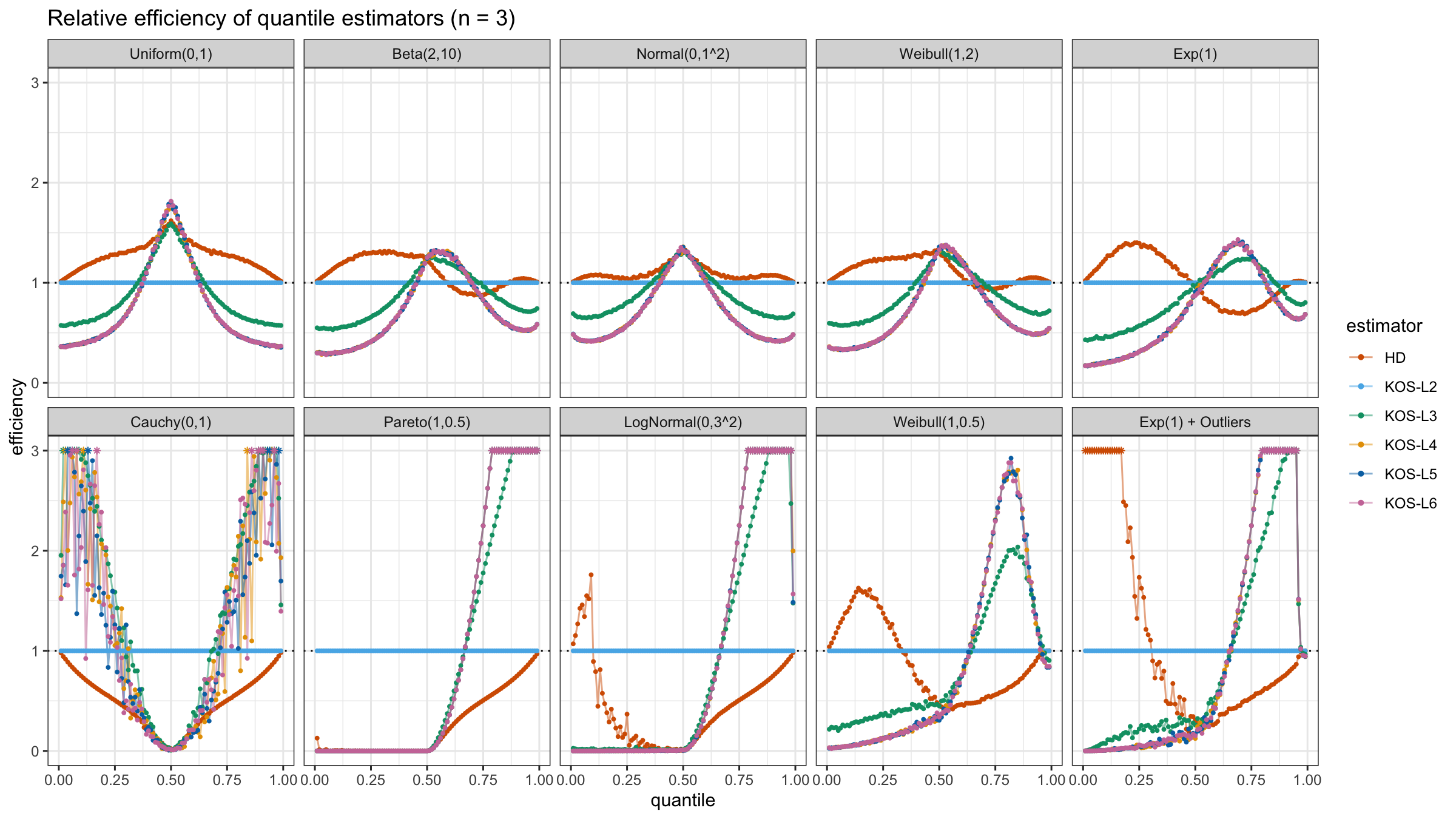
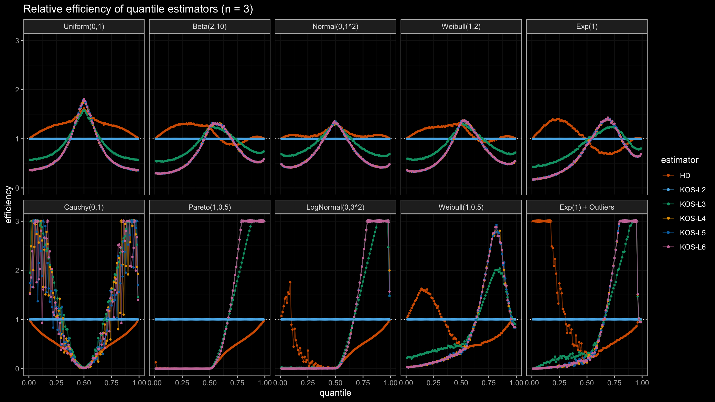
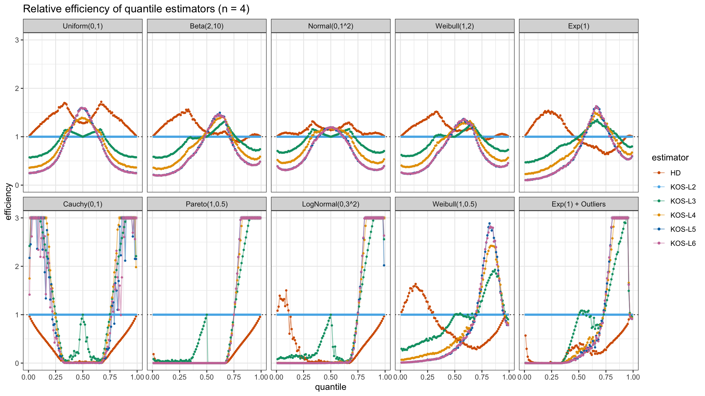
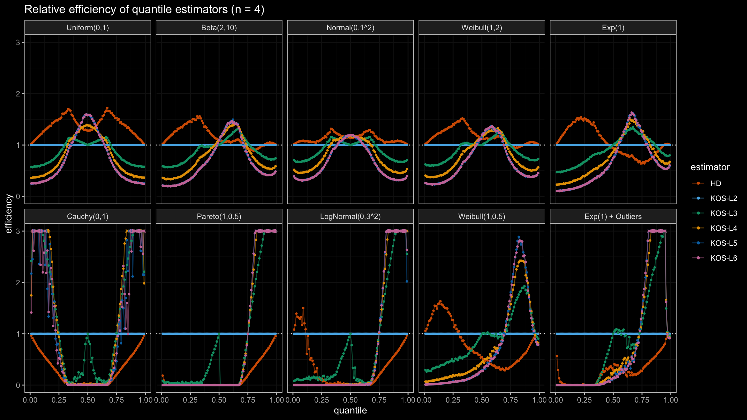
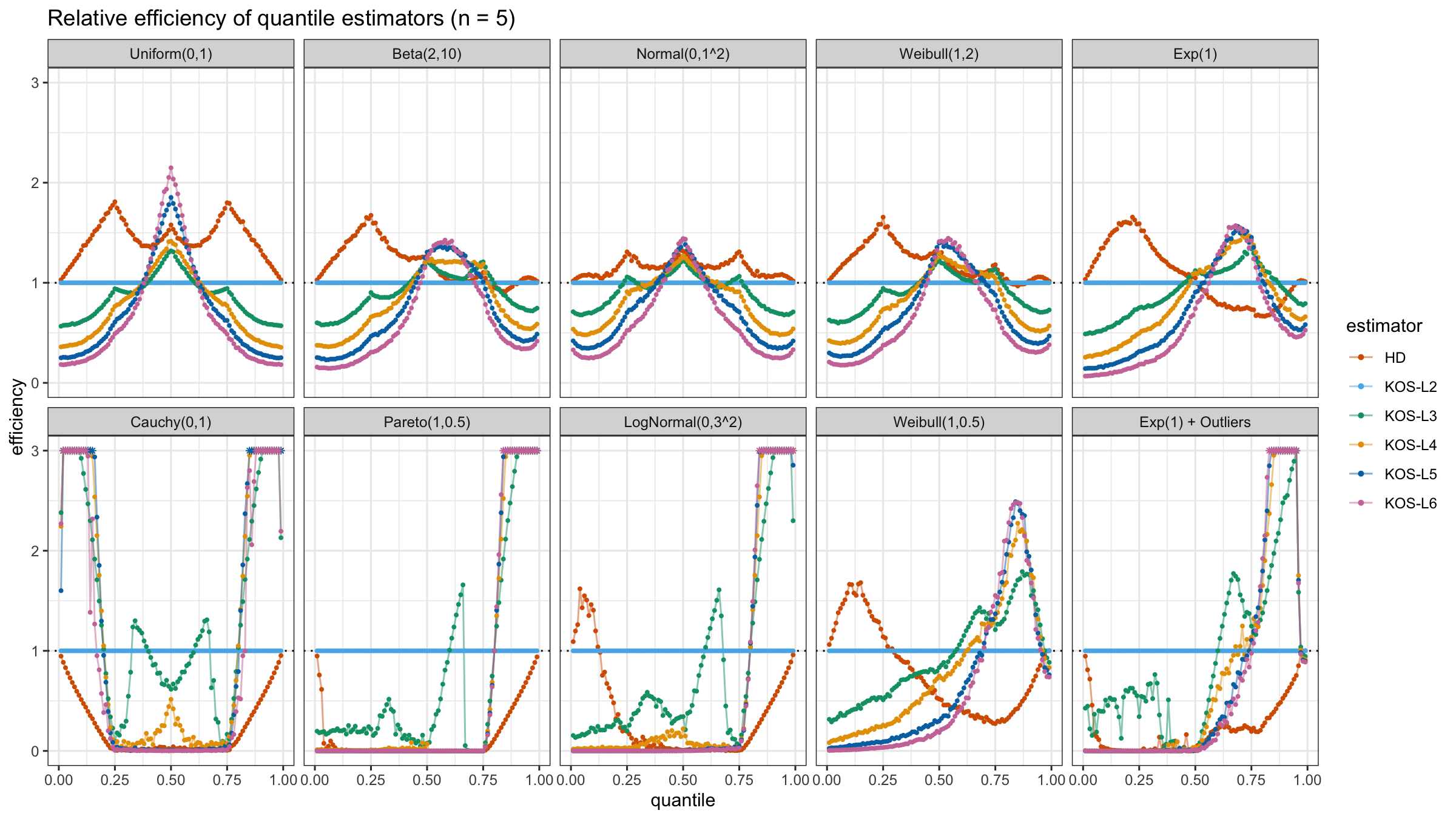
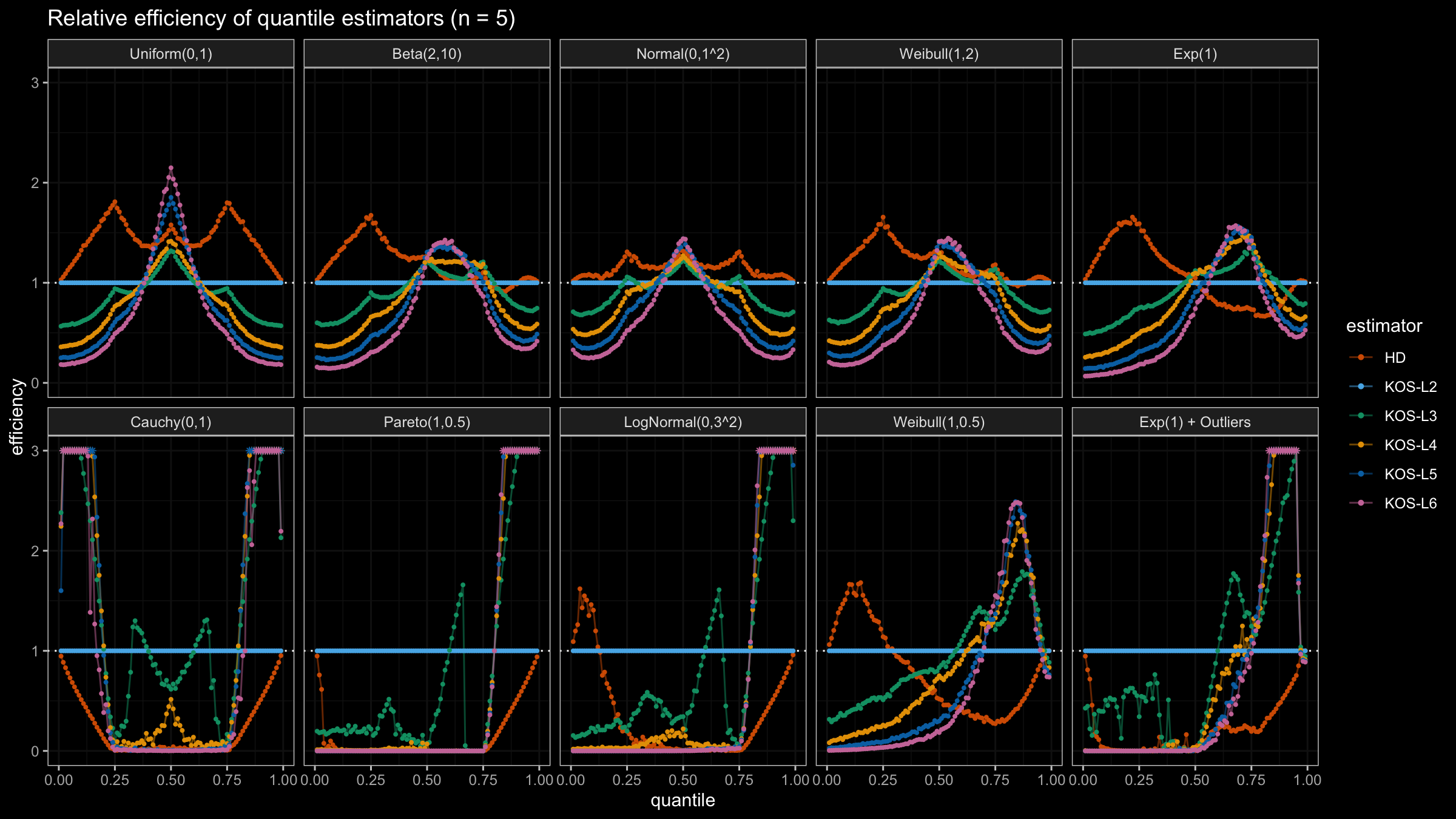
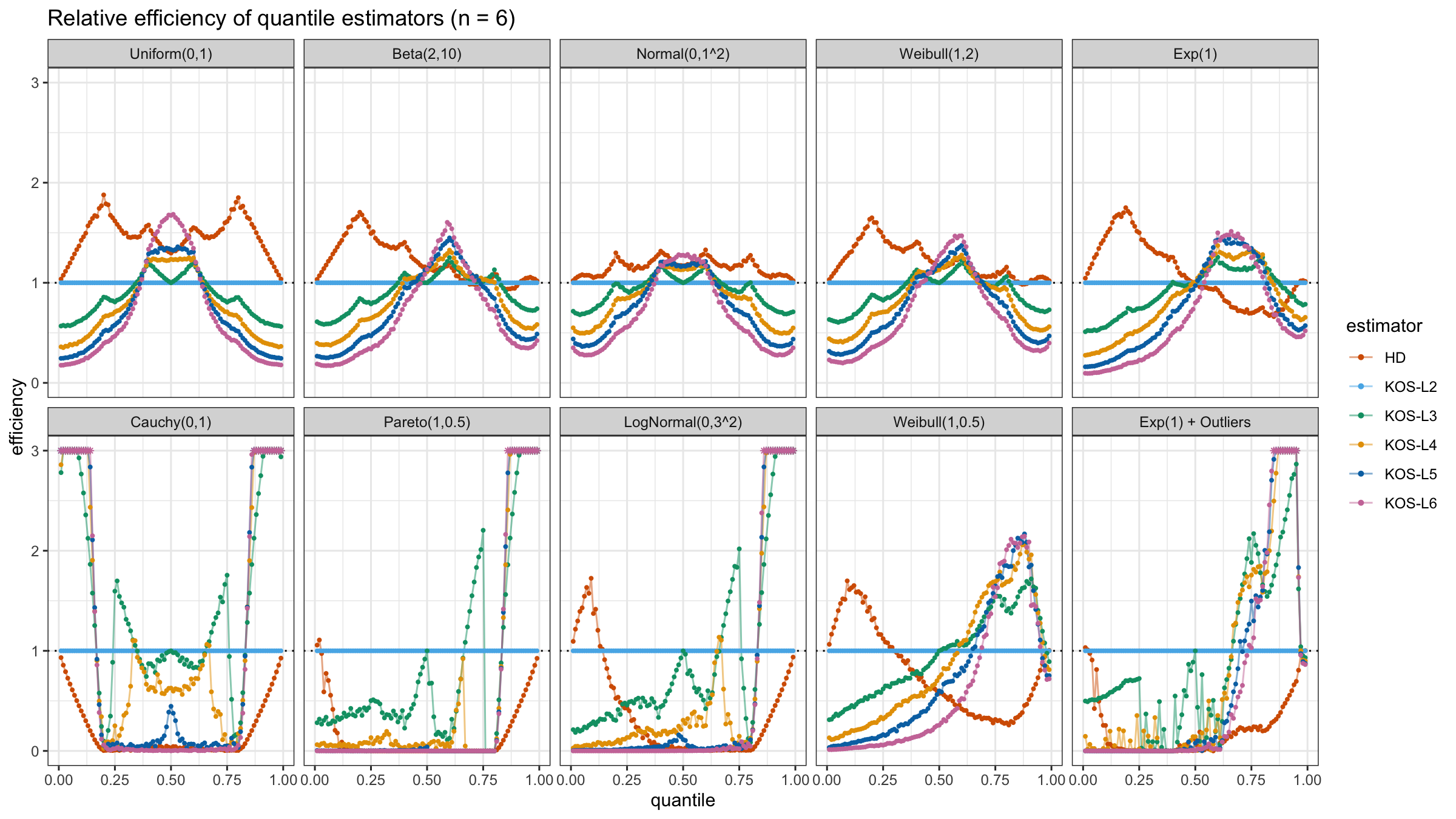
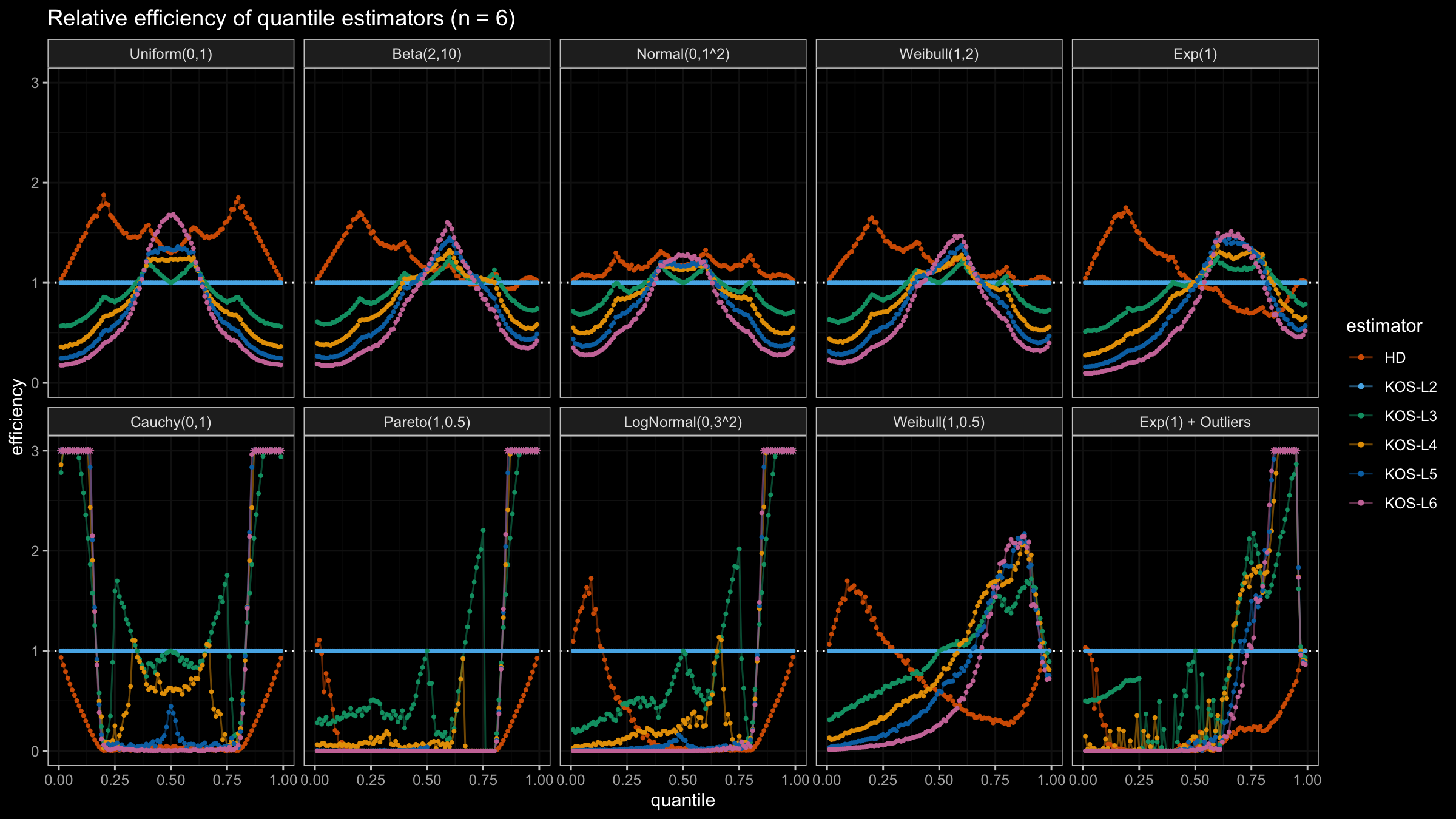
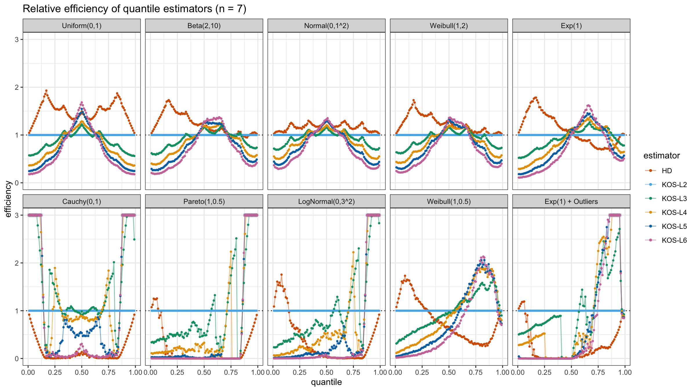
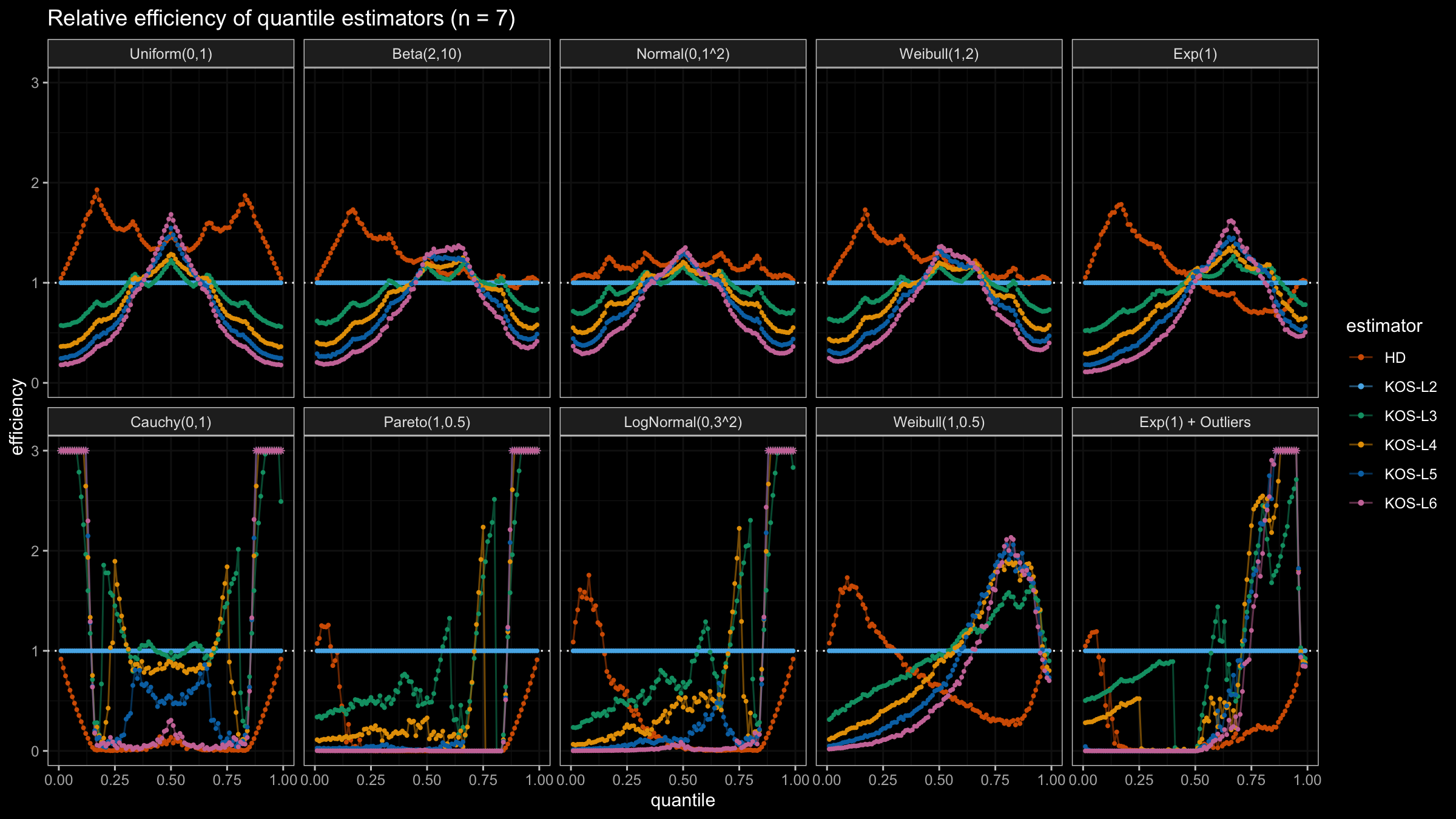
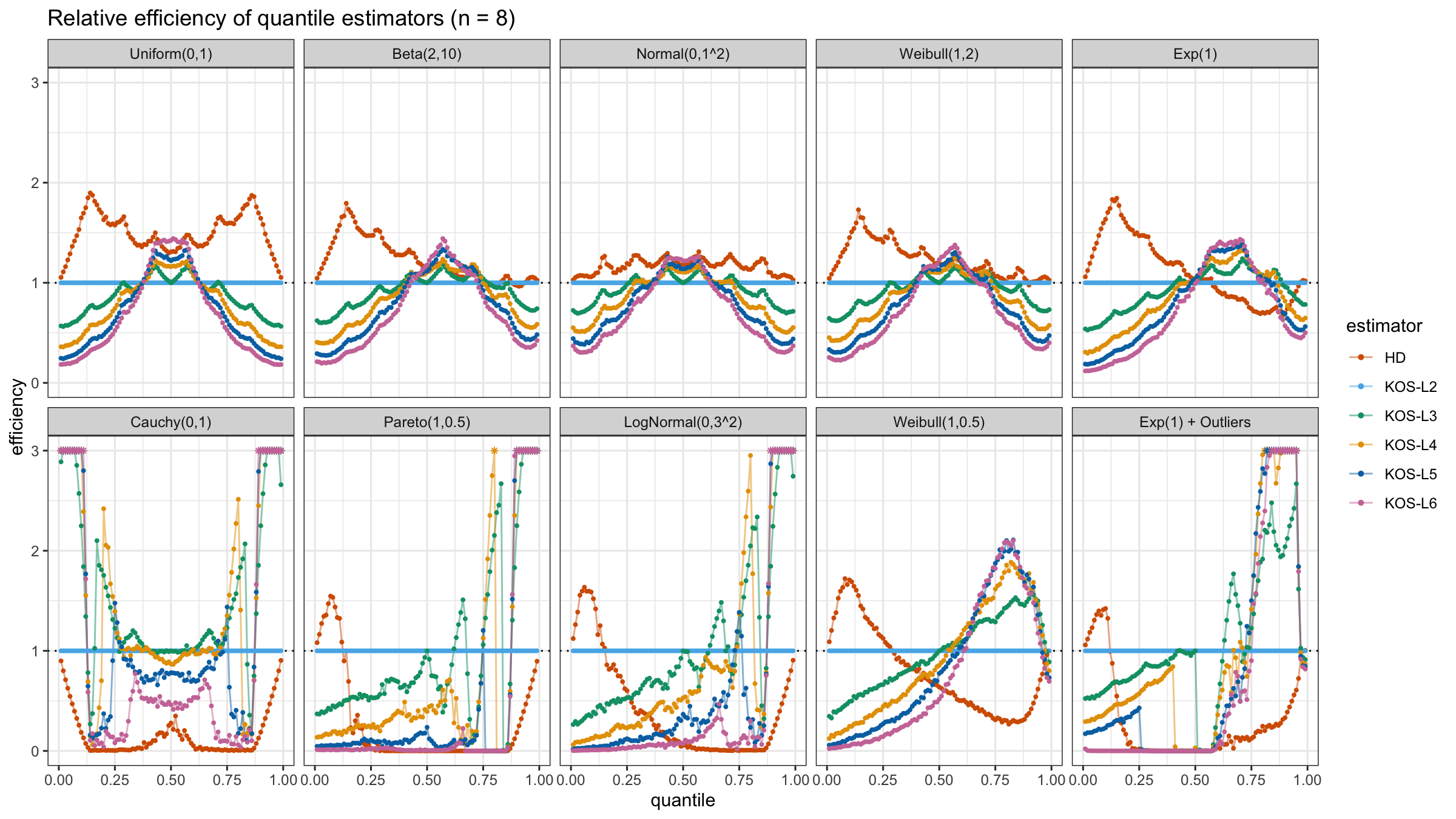
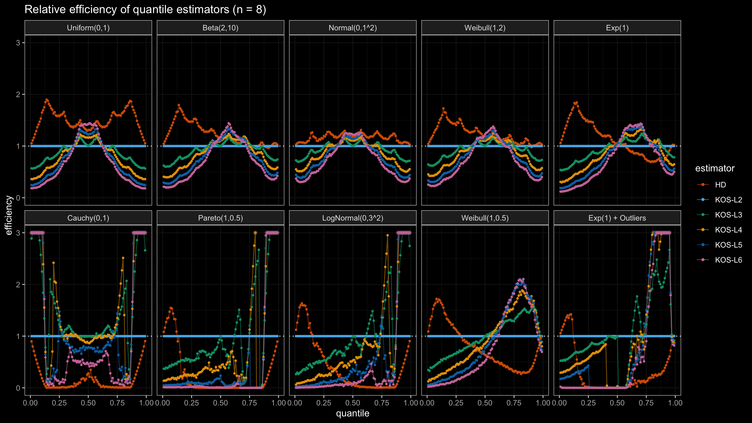
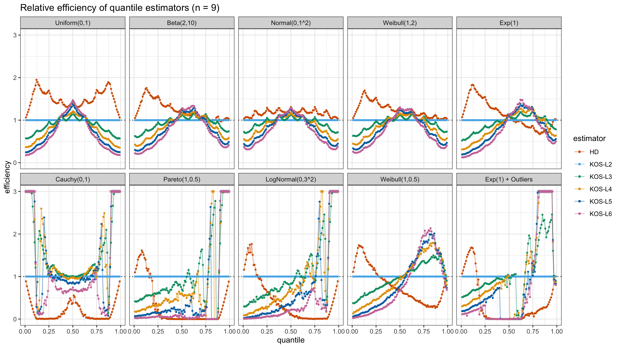
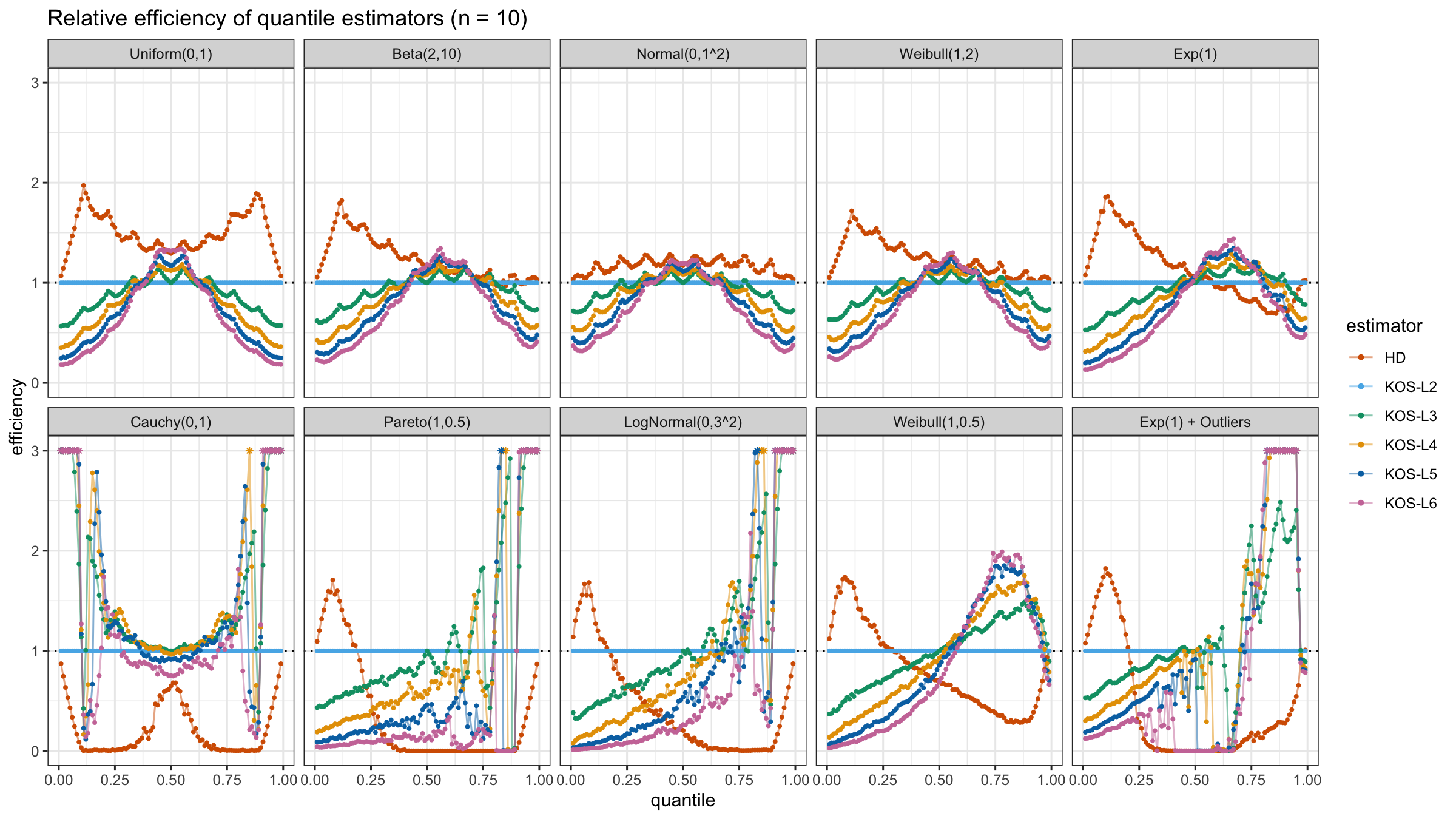
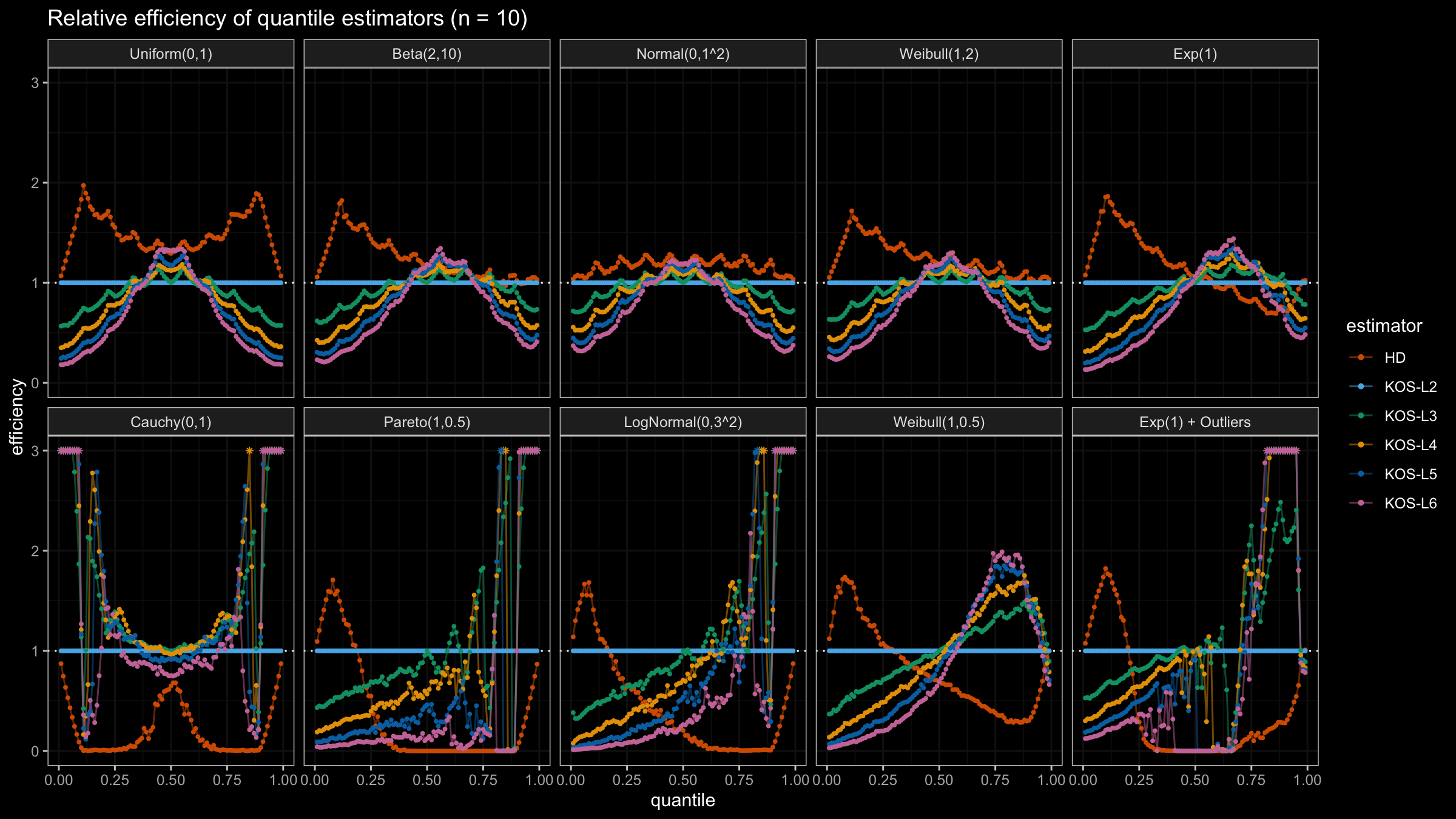
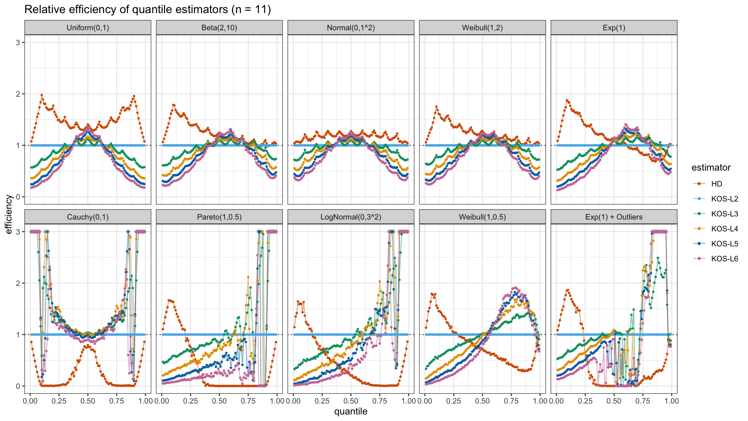
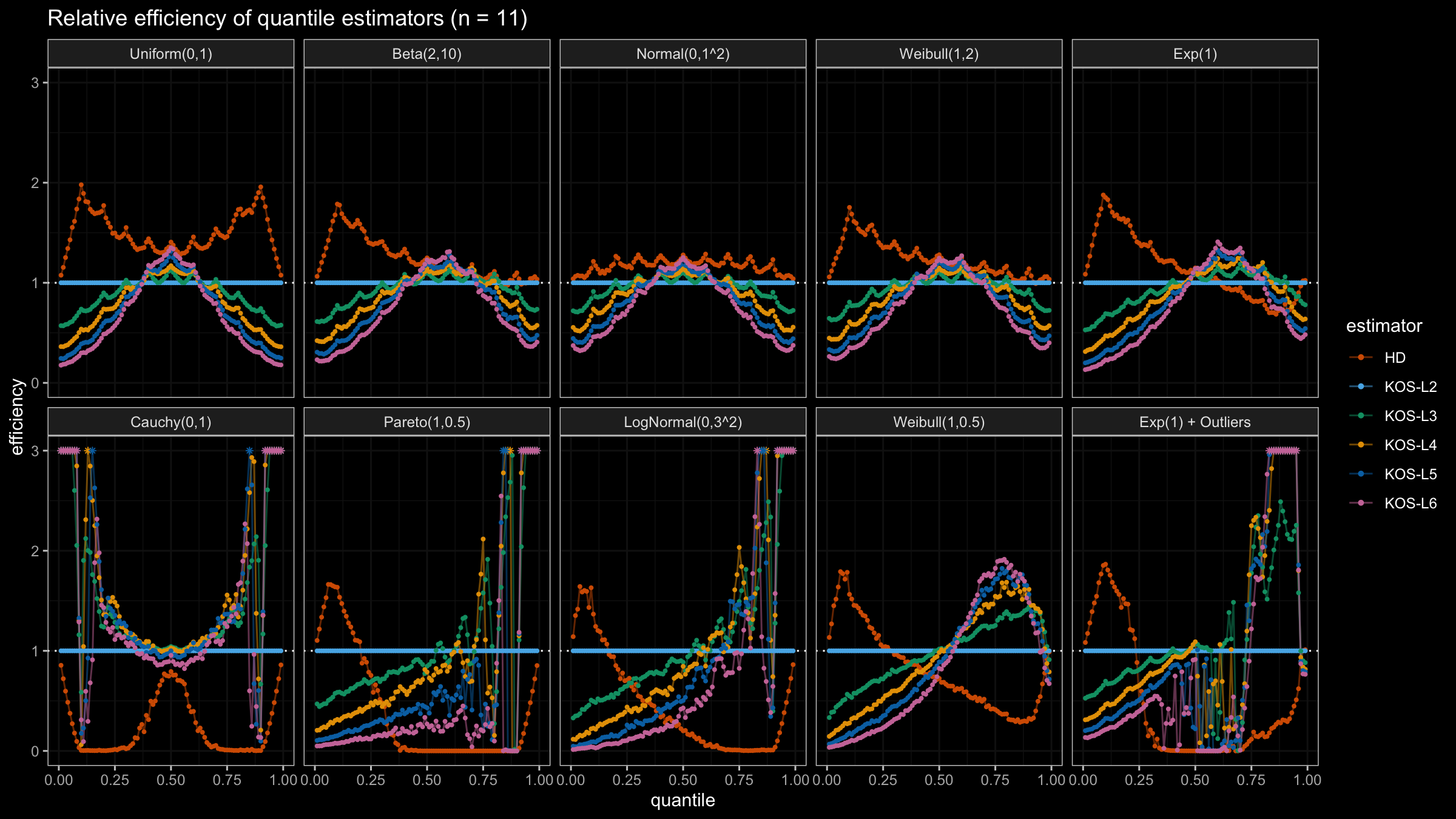
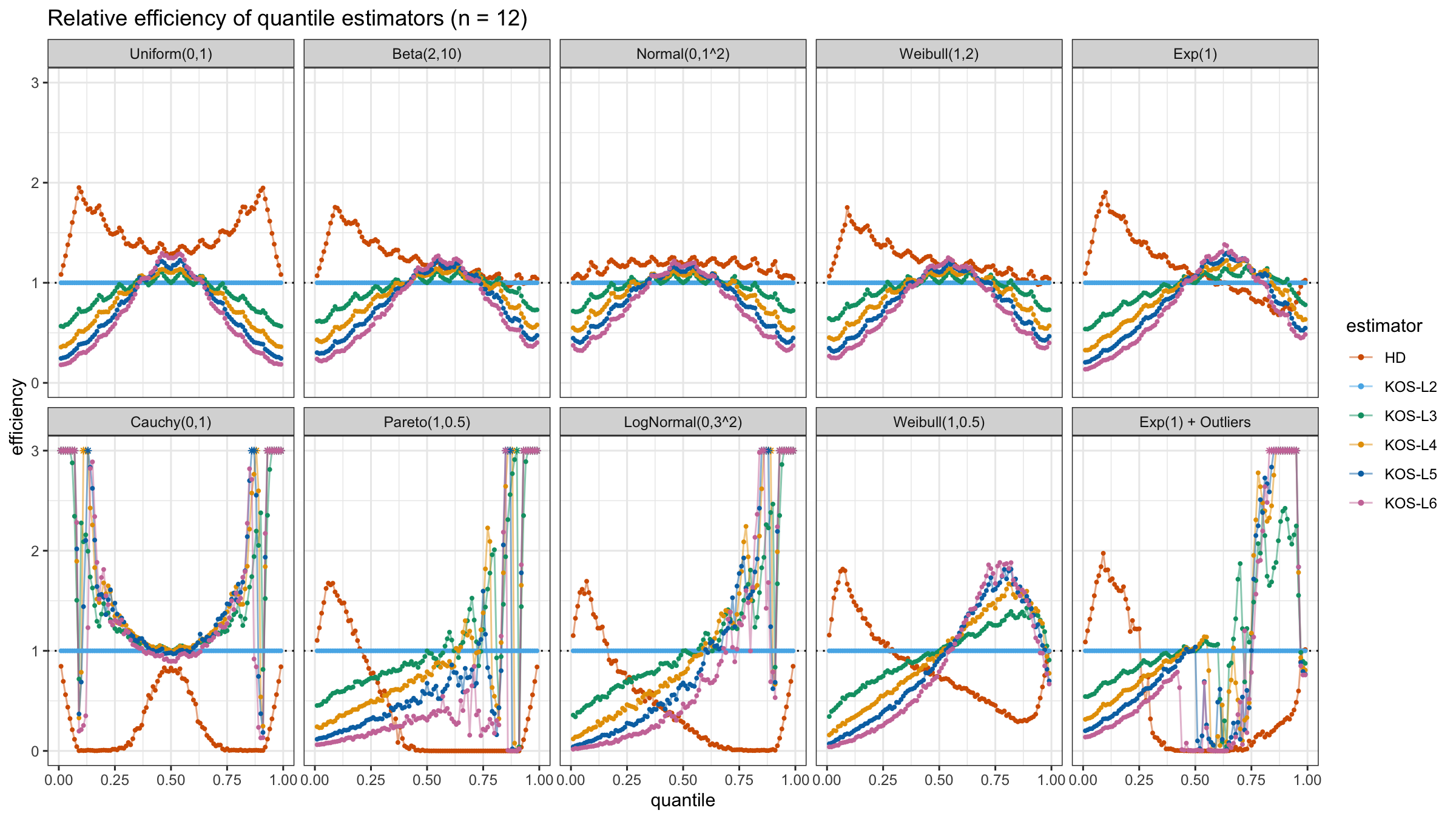
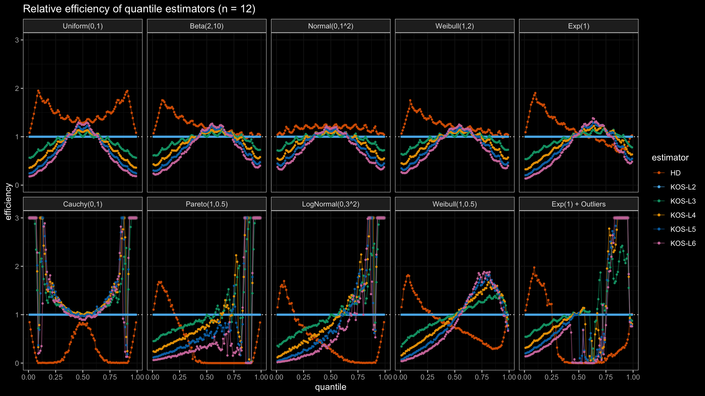
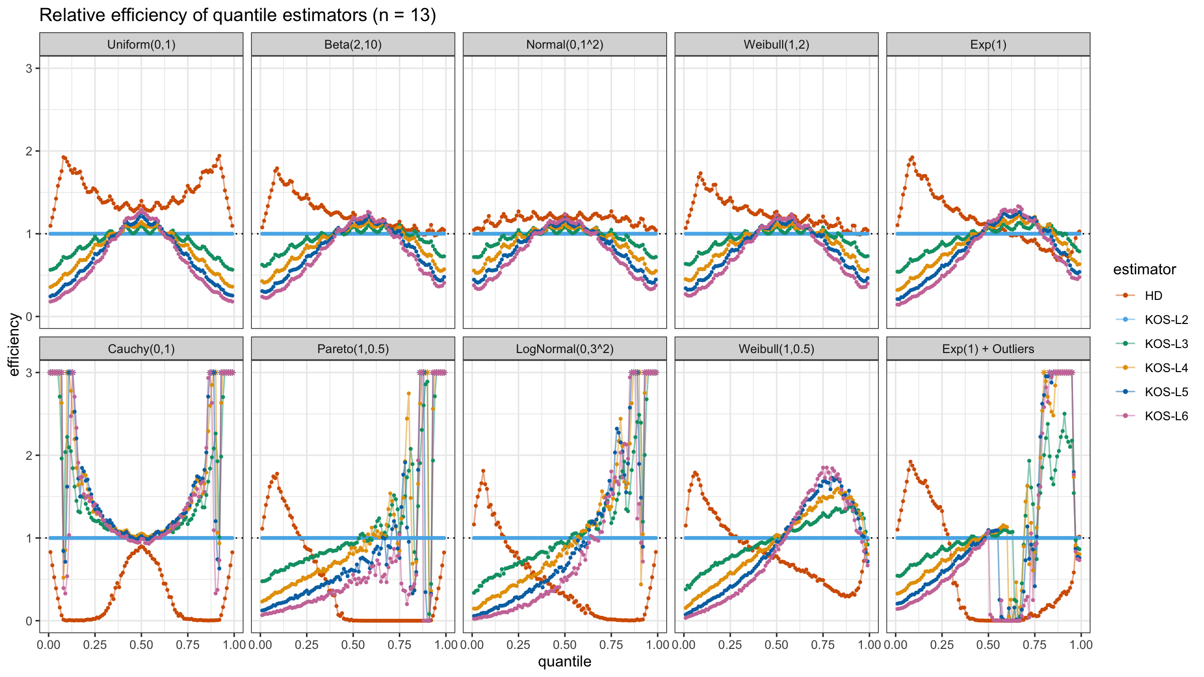
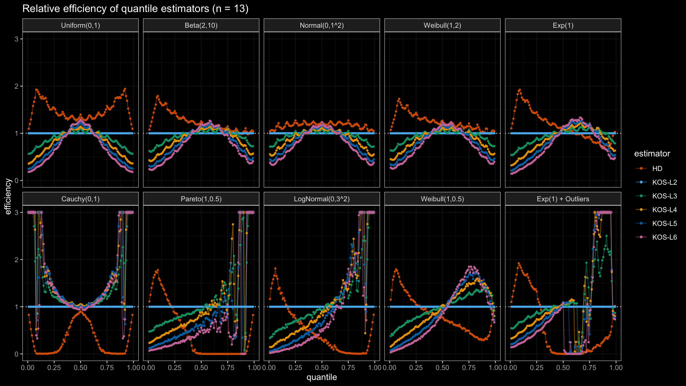
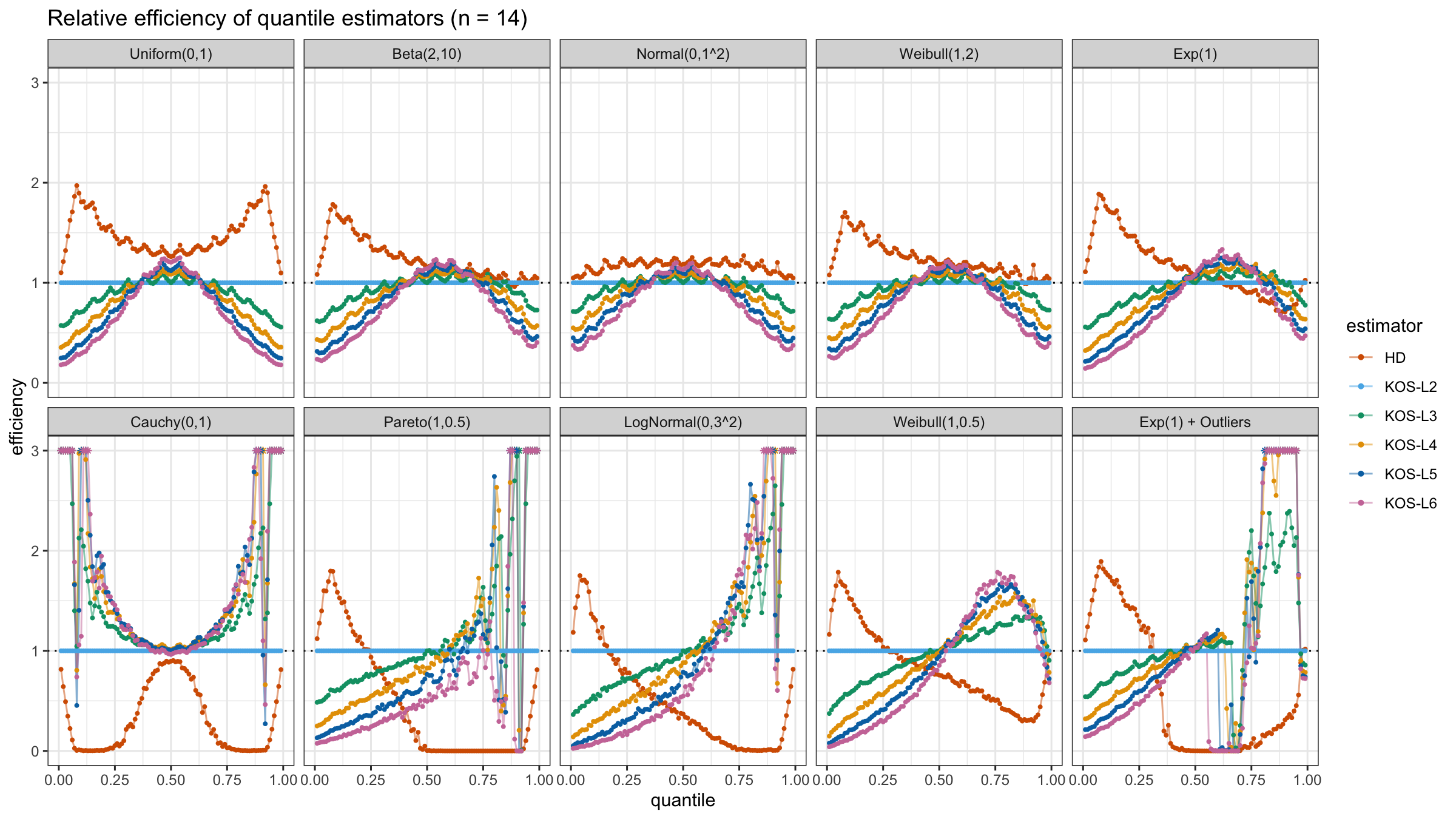
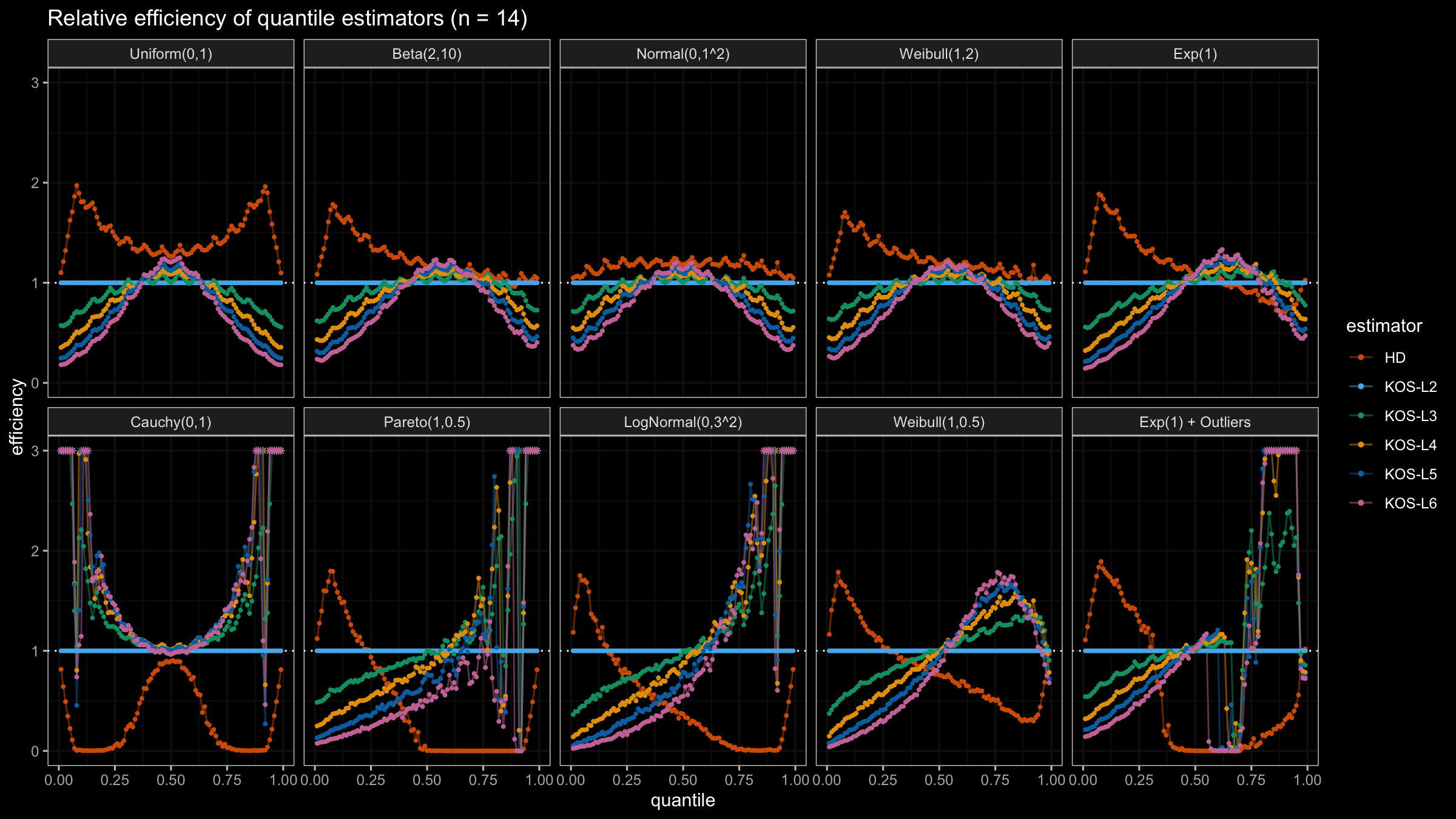
We are going to take the same simulation setup that was declared in this post. Briefly speaking, we evaluate the classic MSE-based relative statistical efficiency of different quantile estimators on samples from different light-tailed and heavy-tailed distributions using the classic Hyndman-Fan Type 7 quantile estimator as the baseline.

Here is the animated version of the simulations (the considered estimators based on k order statistics are denoted as “KOS-Lk”):

And here are static images of the result for different sample sizes:

Conclusion

As I said in the beginning, the statistical efficiency of the suggested quantile estimators is not so impressive. However, it seems there is a relevant use-case for such estimators: symmetric light-tailed distribution + small samples + median estimations. In this case, the suggested estimators are outperforming not only the classic Hyndman-Fan Type 7 quantile estimators but also the Harrell-Davis quantile estimator.

In the next post, we will try another weighted function that is going to provide more impressive results.