Quantile estimators based on k order statistics, Part 3: Playing with the Beta function

In the previous two posts, I discussed the idea of quantile estimators based on k order statistics. A already covered the motivation behind this idea and the statistical efficiency of such estimators using the extended Hyndman-Fan equations as a weight function. Now it’s time to experiment with the Beta function as a primary way to aggregate k order statistics into a single quantile estimation!

All posts from this series:

• Quantile estimators based on k order statistics, Part 1: Motivation (August 3, 2021)
• Quantile estimators based on k order statistics, Part 2: Extending Hyndman-Fan equations (August 10, 2021)
• Quantile estimators based on k order statistics, Part 3: Playing with the Beta function (August 17, 2021)
• Quantile estimators based on k order statistics, Part 4: Adopting trimmed Harrell-Davis quantile estimator (August 24, 2021)
• Quantile estimators based on k order statistics, Part 5: Improving trimmed Harrell-Davis quantile estimator (August 31, 2021)
• Quantile estimators based on k order statistics, Part 6: Continuous trimmed Harrell-Davis quantile estimator (September 7, 2021)
• Quantile estimators based on k order statistics, Part 7: Optimal threshold for the trimmed Harrell-Davis quantile estimator (September 14, 2021)
• Quantile estimators based on k order statistics, Part 8: Winsorized Harrell-Davis quantile estimator (September 21, 2021)

The approach

The general idea is the same that was used in the previous post. We express the estimation of the $p^\textrm{th}$ quantile as follows:

$$ \begin{gather*} q_p = \sum_{i=1}^{n} W_{i} \cdot x_i,\\ W_{i} = F(r_i) - F(l_i),\\ l_i = (i - 1) / n, \quad r_i = i / n, \end{gather*} $$

where F is a CDF function of a specific distribution. The distribution has non-zero PDF only inside a window $[L_k, R_k]$ that covers at most k order statistics:

$$ F(u) = \left\{ \begin{array}{lcrcllr} 0 & \textrm{for} & & & u & < & L_k, \\ G\Big((u - L_k)/(R_k-L_k)\Big) & \textrm{for} & L_k & \leq & u & \leq & R_k, \\ 1 & \textrm{for} & R_k & < & u, & & \end{array} \right. $$ $$ L_k = (h - 1) / (n - 1) \cdot (n - (k - 1)) / n, \quad R_k = L_k + (k-1)/n, $$ $$ h = (n - 1)p + 1. $$

Now we just have to define the $G: [0;1] \to [0;1]$ function that defines $F$ values inside the window. In the previous post, where we used the extension of Hyndman-Fan Type 7 equation, we used just the most simple linear function:

$$ G_{HF7}(u) = u. $$

In this post, we are going to try the Beta distribution (which is used in the Harrell-Davis quantile estimator). The CDF of the Beta distribution is the regularized incomplete beta function) $I_x(\alpha, \beta)$. We will try this idea with $\alpha=kp, \beta = k(1-p)$:

$$ G(u) = I_u(kp, k(1-p)). $$

With such values, the suggested estimator becomes the exact copy of the Harrell-Davis quantile estimator for $k=n+1$. Let’s perform some numerical simulations to check the statistical efficiency of this estimator.

Numerical simulations

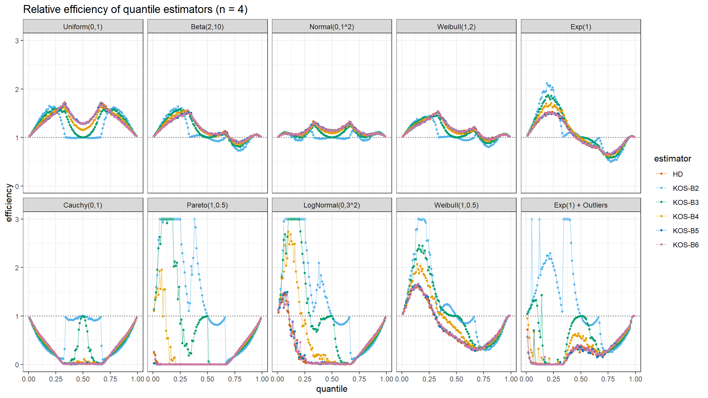
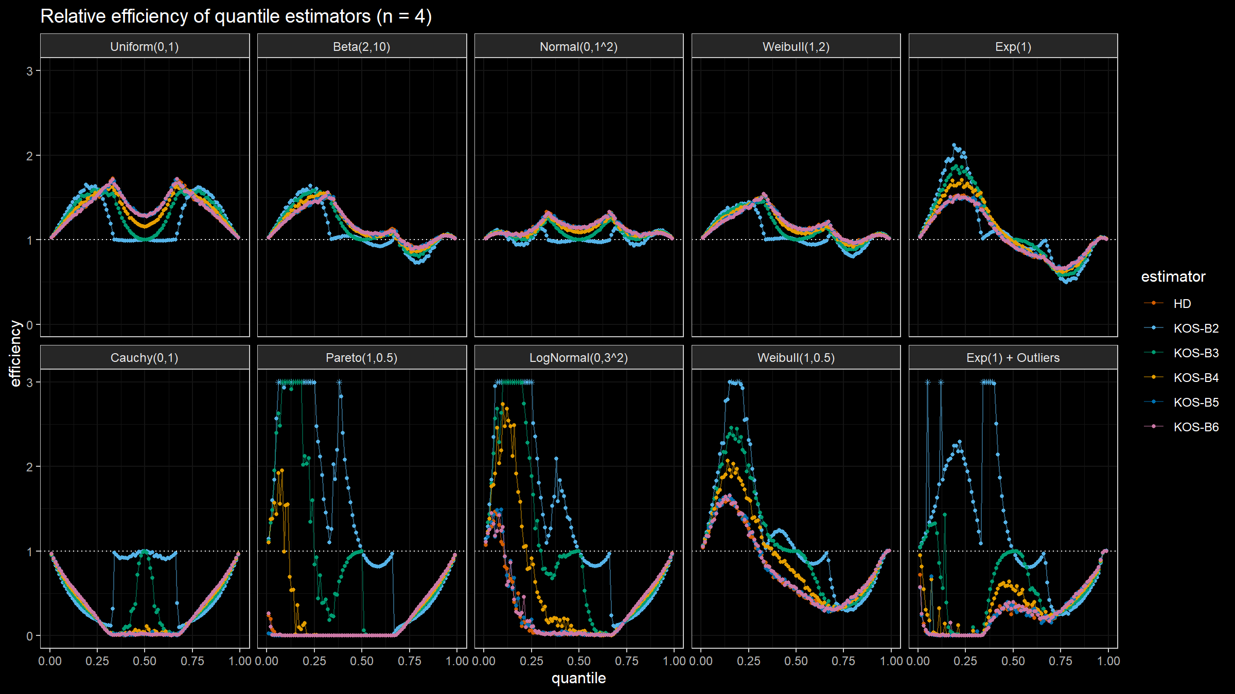
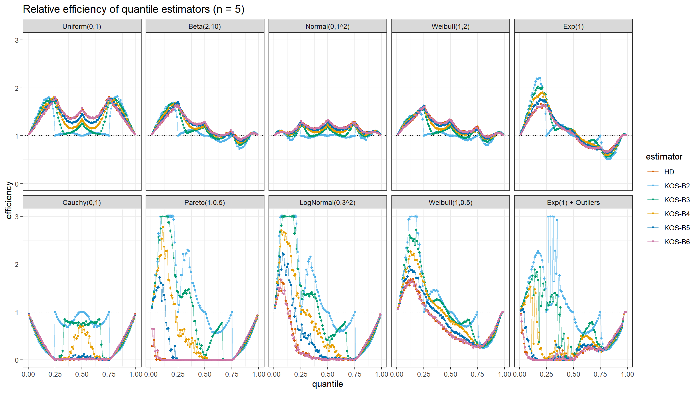
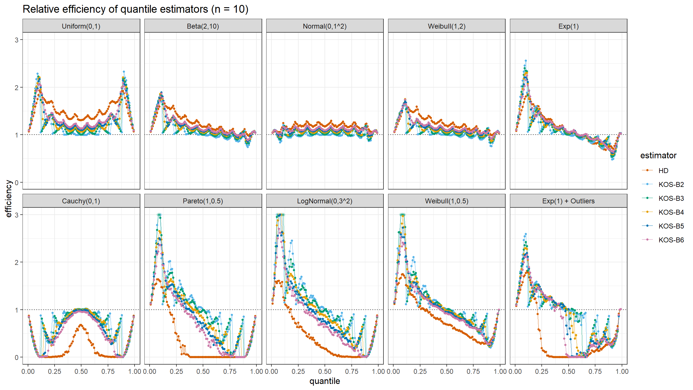
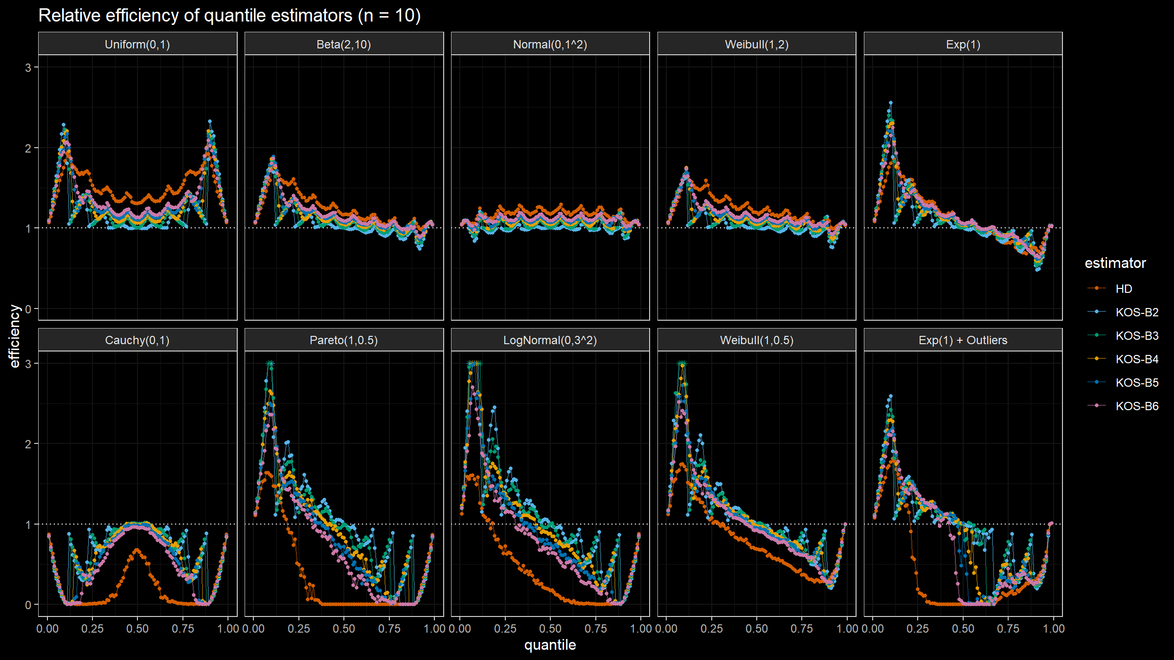
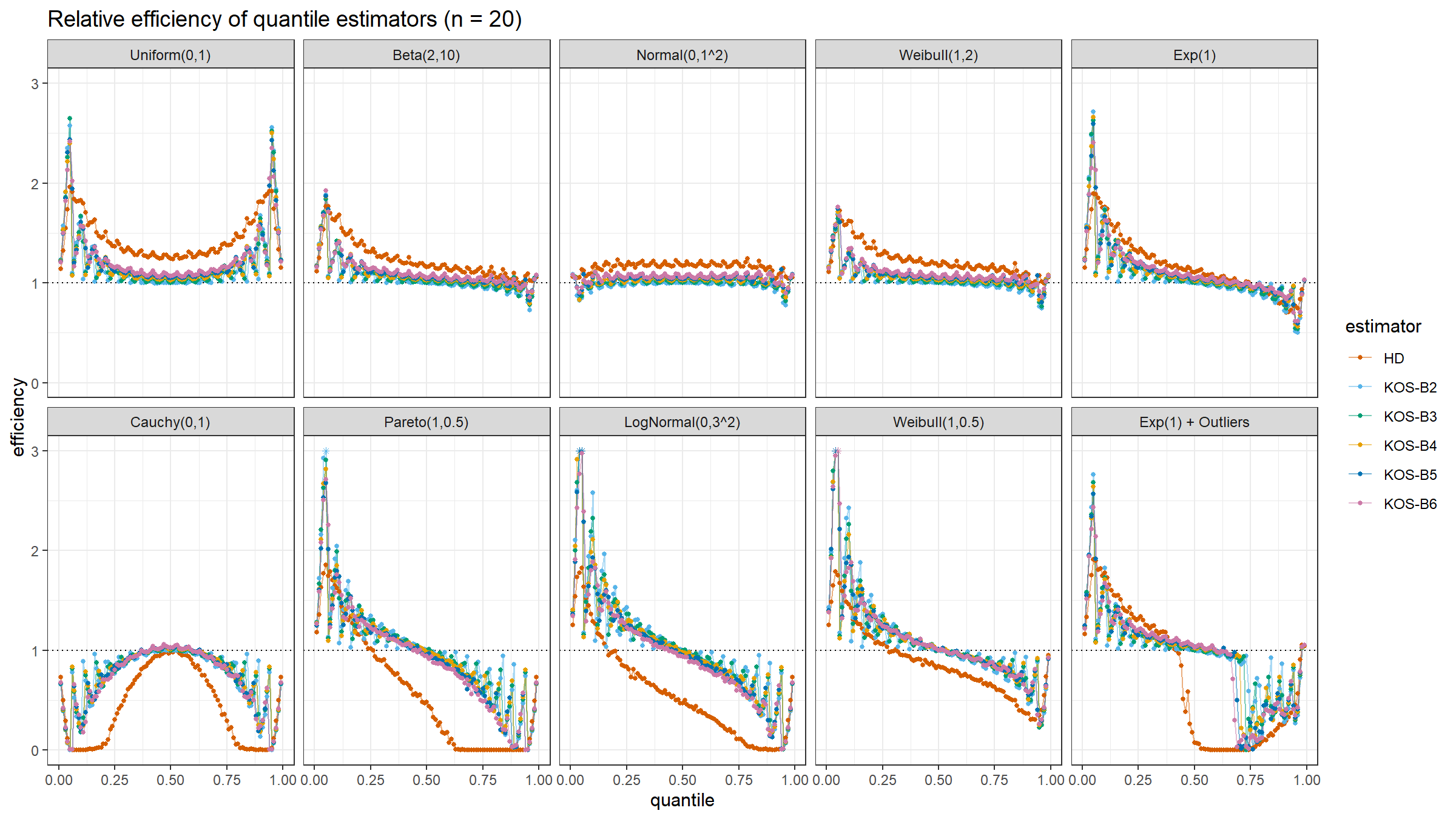
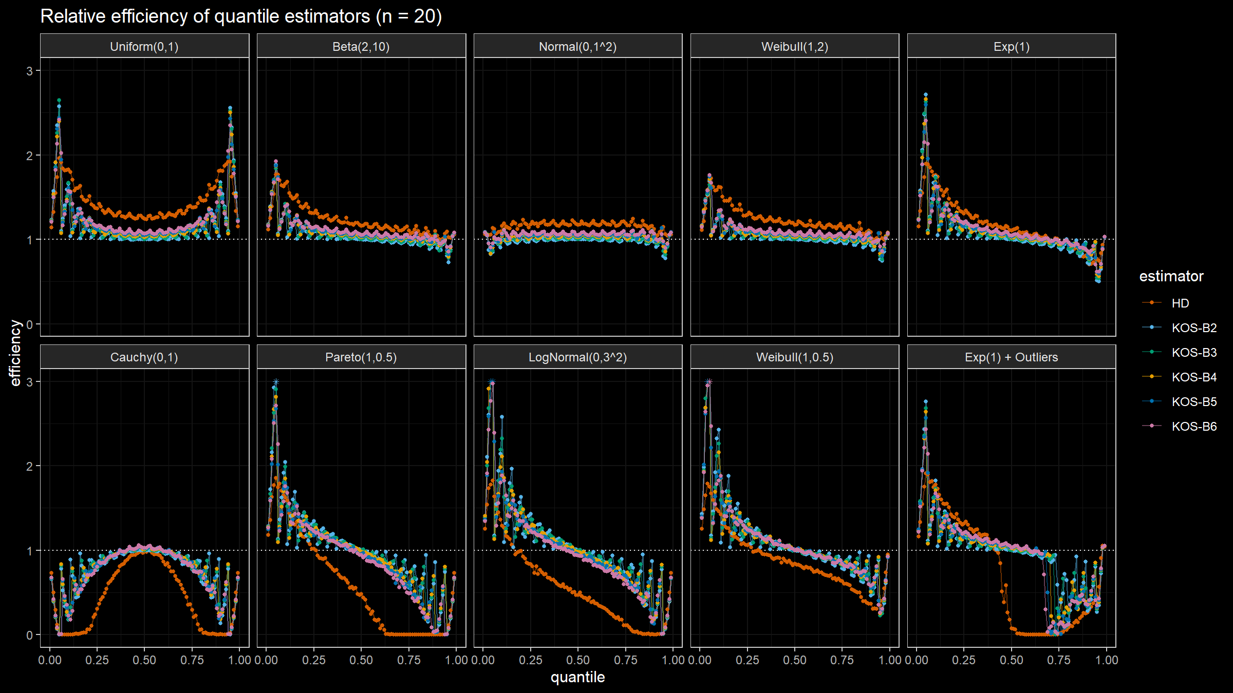
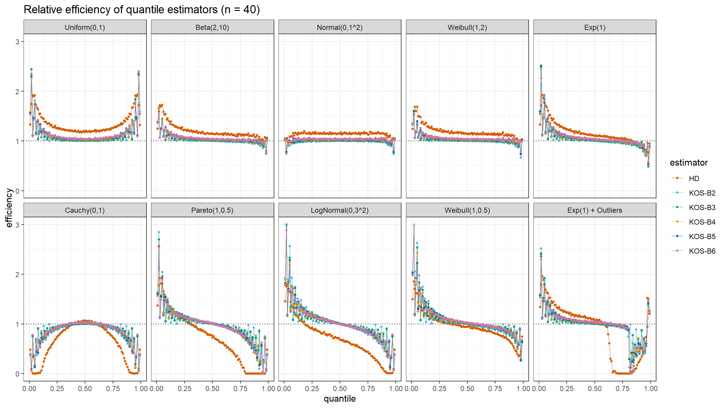
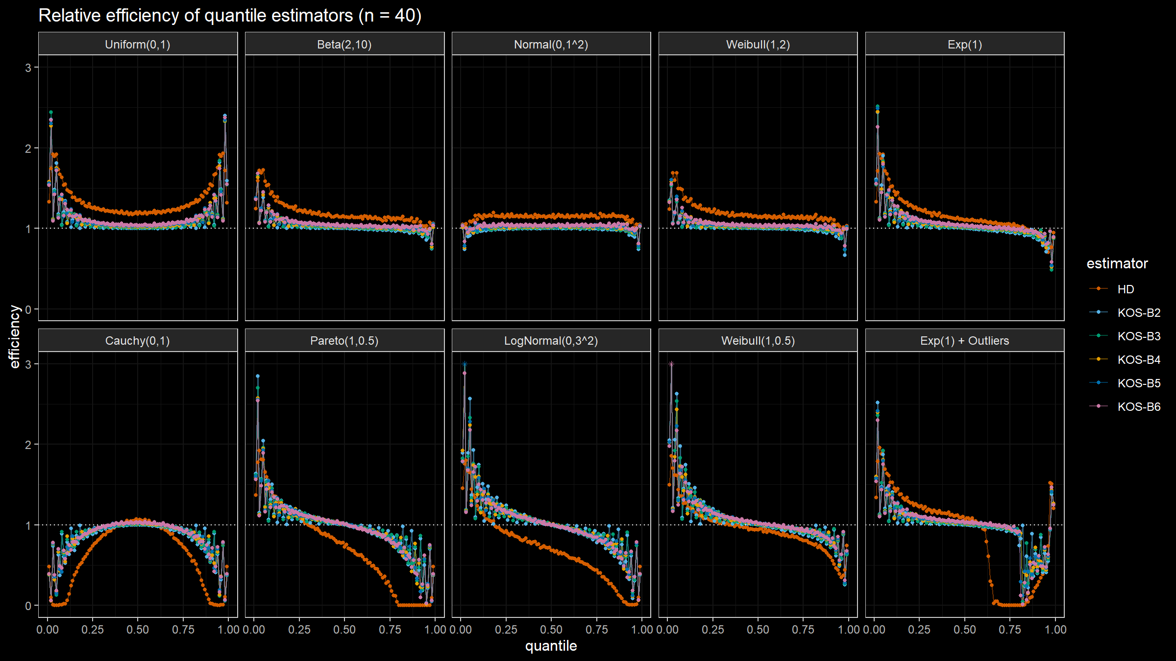
We are going to take the same simulation setup that was declared in this post. Briefly speaking, we evaluate the classic MSE-based relative statistical efficiency of different quantile estimators on samples from different light-tailed and heavy-tailed distributions using the classic Hyndman-Fan Type 7 quantile estimator as the baseline.

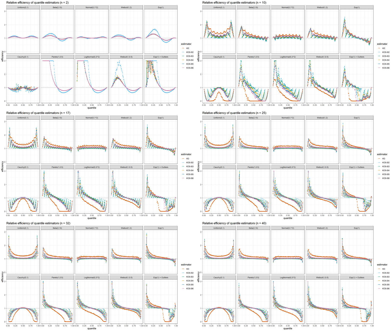
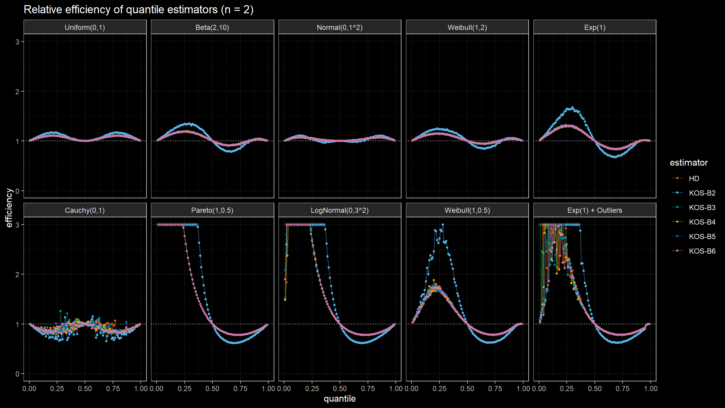
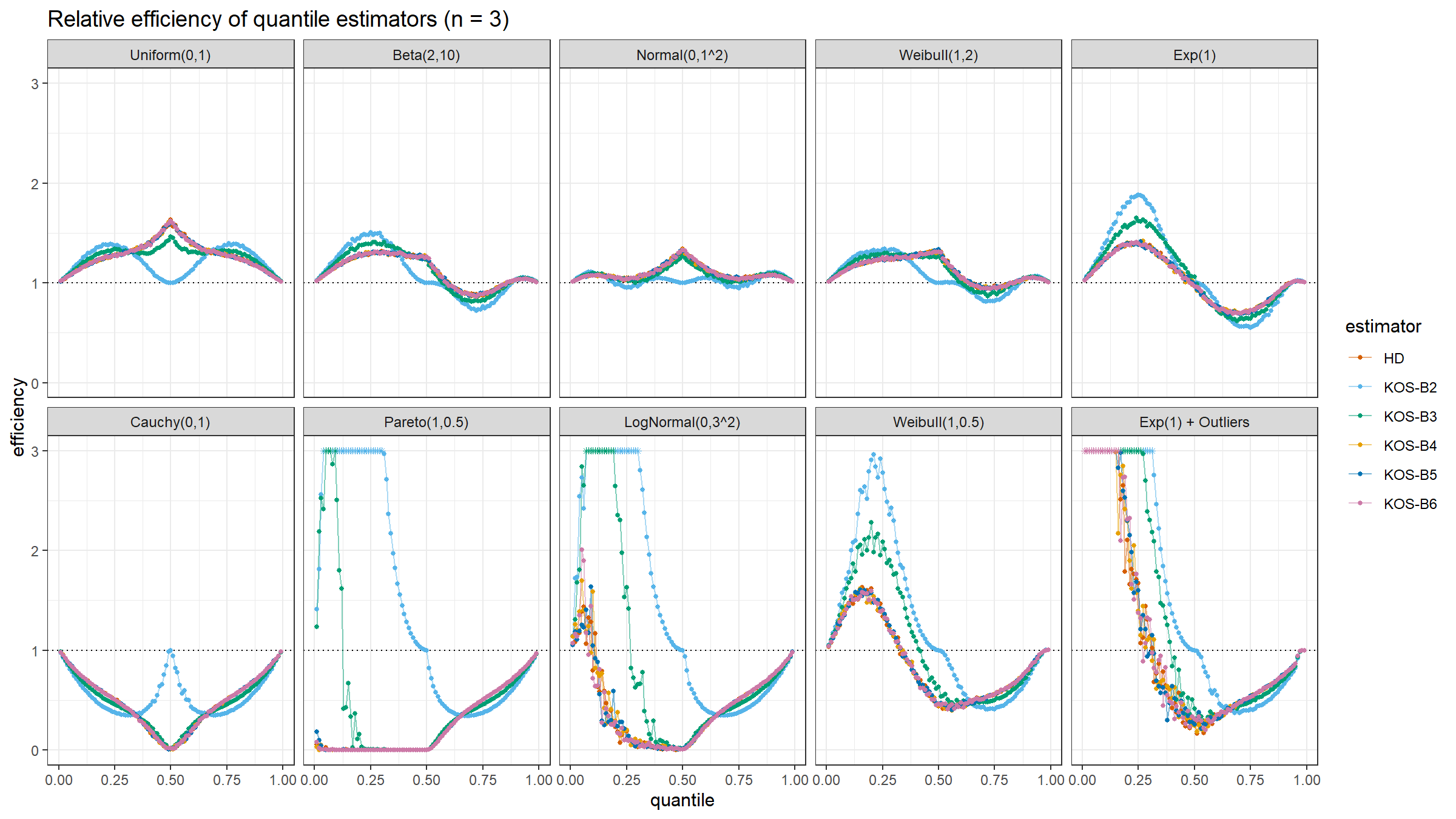
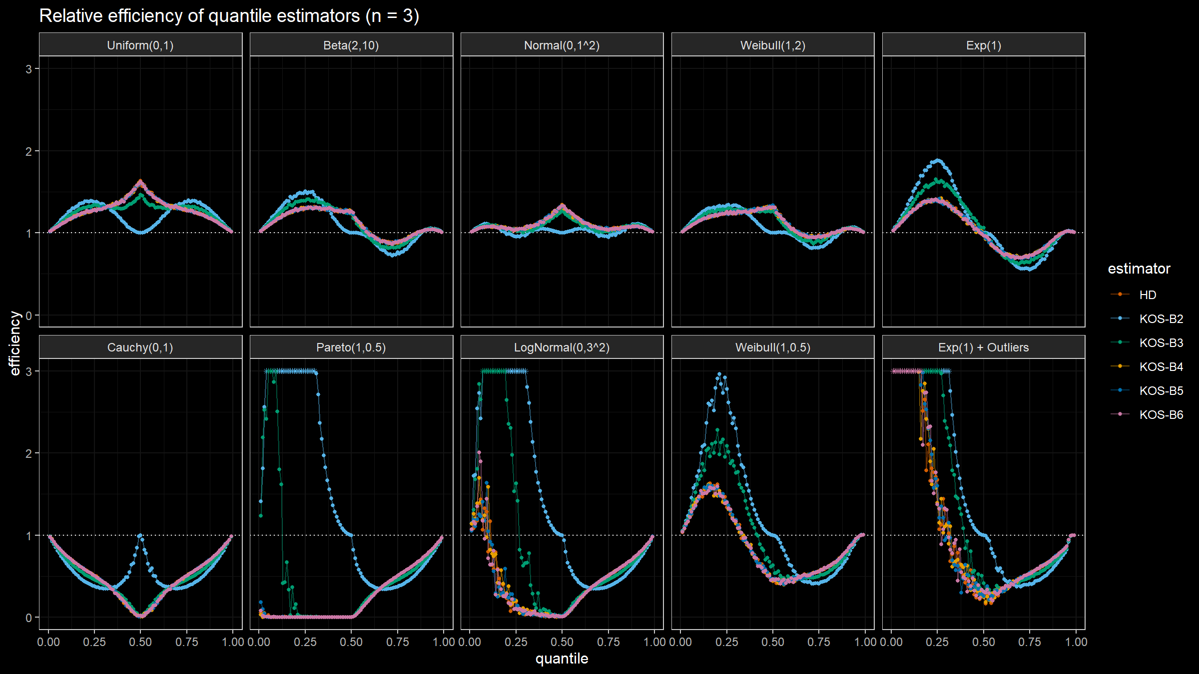
Here is the animated version of the simulations (the considered estimators based on k order statistics are denoted as “KOS-Bk”):

And here are static images of the result for different sample sizes:

Conclusion

In this post, we discussed a quantile estimator that is based on k order statistics aggregated using the Beta function. It seems that this estimator is a good step in the right direction: it’s better than the traditional Hyndman-Fan Type 7 quantile estimator for the samples from light-tailed distributions (however, it’s worse than the Harrell-Davis quantile estimator). Also, it’s more robust than the Harrell-Davis quantile estimator in the case of heavy-tailed distributions. Moreover, we could specify the desired breakdown point by customizing the k value.

In the next post, we are going to try one more weight function.