Quantile estimators based on k order statistics, Part 4: Adopting trimmed Harrell-Davis quantile estimator

In the previous posts, I discussed various aspects of quantile estimators based on k order statistics. I already tried a few weight functions that aggregate the sample values to the quantile estimators (see posts about an extension of the Hyndman-Fan Type 7 equation and about adjusted regularized incomplete beta function). In this post, I continue my experiments and try to adopt the trimmed modifications of the Harrell-Davis quantile estimator to this approach.

All posts from this series:

• Quantile estimators based on k order statistics, Part 1: Motivation (August 3, 2021)
• Quantile estimators based on k order statistics, Part 2: Extending Hyndman-Fan equations (August 10, 2021)
• Quantile estimators based on k order statistics, Part 3: Playing with the Beta function (August 17, 2021)
• Quantile estimators based on k order statistics, Part 4: Adopting trimmed Harrell-Davis quantile estimator (August 24, 2021)
• Quantile estimators based on k order statistics, Part 5: Improving trimmed Harrell-Davis quantile estimator (August 31, 2021)
• Quantile estimators based on k order statistics, Part 6: Continuous trimmed Harrell-Davis quantile estimator (September 7, 2021)
• Quantile estimators based on k order statistics, Part 7: Optimal threshold for the trimmed Harrell-Davis quantile estimator (September 14, 2021)
• Quantile estimators based on k order statistics, Part 8: Winsorized Harrell-Davis quantile estimator (September 21, 2021)

The approach

The general idea is the same that was used in one of the previous posts. We express the estimation of the $p^\textrm{th}$ quantile as follows:

$$ \begin{gather*} q_p = \sum_{i=1}^{n} W_{i} \cdot x_i,\\ W_{i} = F(r_i) - F(l_i),\\ l_i = (i - 1) / n, \quad r_i = i / n, \end{gather*} $$

where F is a CDF function of a specific distribution. The distribution has non-zero PDF only inside a window $[L_k, R_k]$ that covers at most k order statistics:

$$ F(u) = \left\{ \begin{array}{lcrcllr} 0 & \textrm{for} & & & u & < & L_k, \\ G(u) & \textrm{for} & L_k & \leq & u & \leq & R_k, \\ 1 & \textrm{for} & R_k & < & u, & & \end{array} \right. $$ $$ L_k = (h - 1) / (n - 1) \cdot (n - (k - 1)) / n, \quad R_k = L_k + (k-1)/n, $$ $$ h = (n - 1)p + 1. $$

Now we just have to define the $G: [0;1] \to [0;1]$ function that defines $F$ values inside the window. We already discussed a few possible options for $G$:

• An extension of Hyndman-Fan Type 7 equation:

$$ G_{HF7}(u) = (u - L_k)/(R_k-L_k). $$

• Adjusted regularized incomplete beta function:

$$ G_{\textrm{Beta}}(u) = I_{(u - L_k)/(R_k-L_k)}(kp, k(1-p)). $$

Now it’s time to try the trimmed modifications of the Harrell-Davis quantile estimator (THD). In order to adjust THD, we should rescale the original regularized incomplete beta function:

$$ G_{\textrm{THD}}(u) = (I_u - I_{L_k}) / (I_{R_k} - I_{L_k}), \quad I_x = I_x(p(n+1), (1-p)(n+1)) $$

With such values, the suggested estimator becomes the exact copy of the Harrell-Davis quantile estimator for $k=n+1$. Let’s perform some numerical simulations to check the statistical efficiency of this estimator.

Numerical simulations

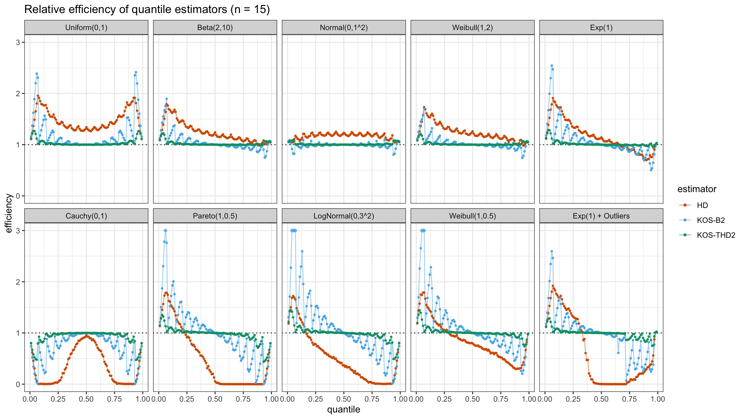
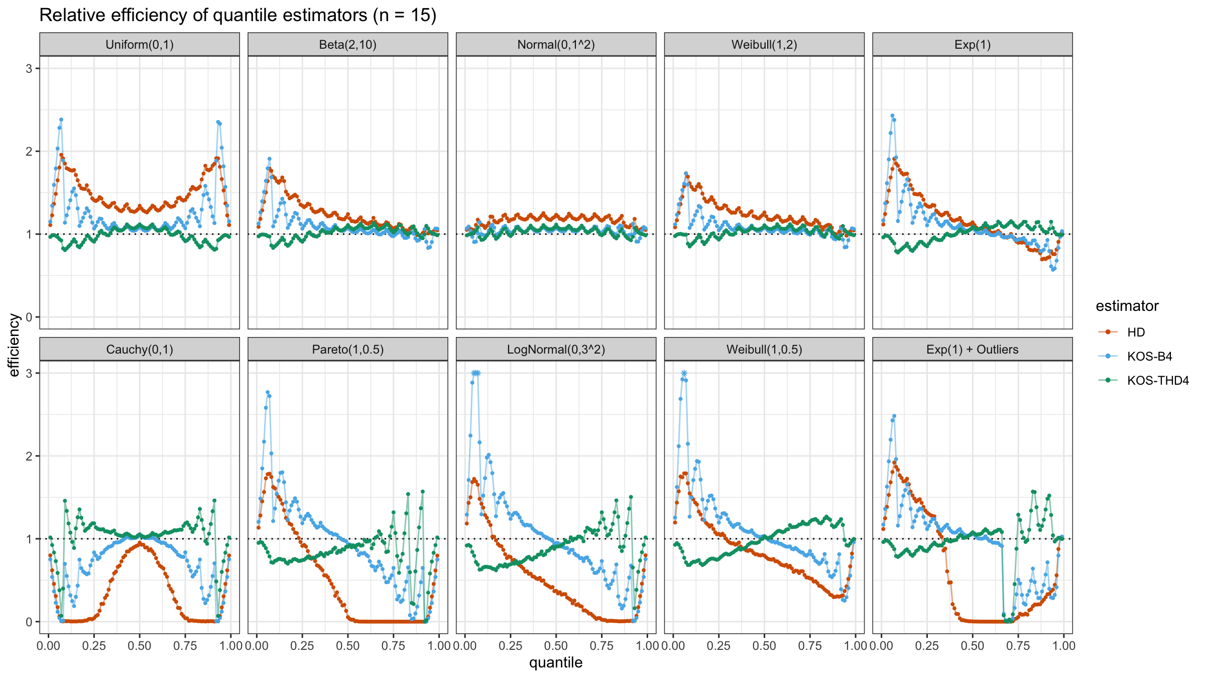
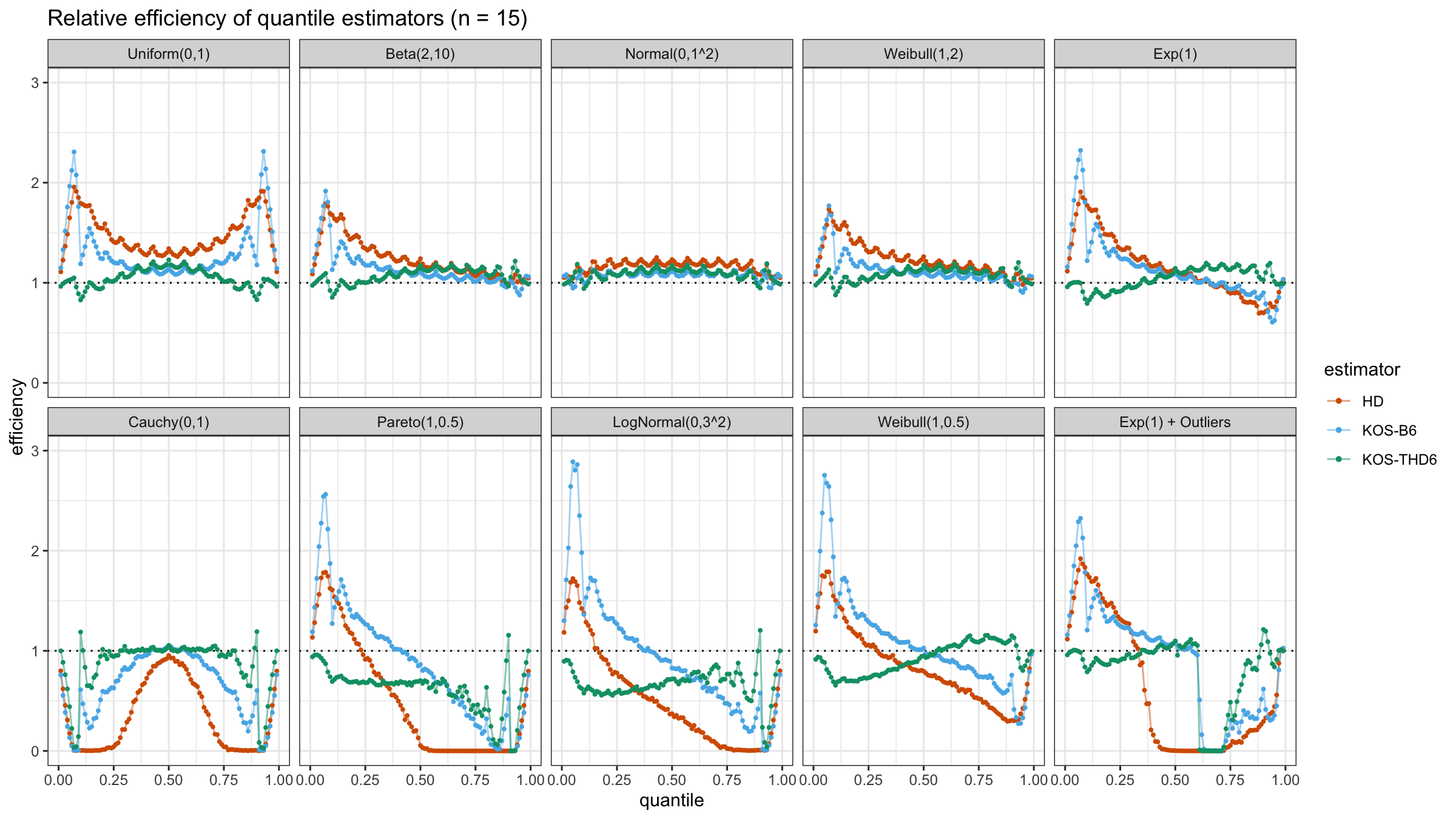
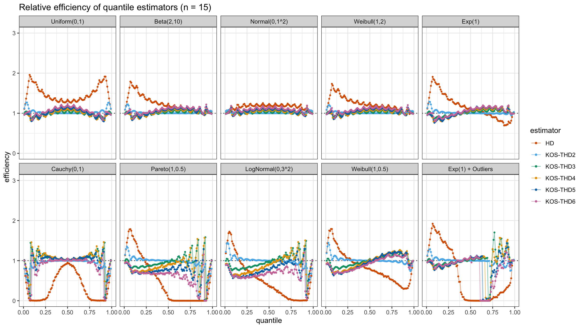
We are going to take the same simulation setup that was declared in this post. Briefly speaking, we evaluate the classic MSE-based relative statistical efficiency of different quantile estimators on samples from different light-tailed and heavy-tailed distributions using the classic Hyndman-Fan Type 7 quantile estimator as the baseline.

The considered estimator based on k order statistics is denoted as “KOS-THDk”. The estimator from the previous post based on the adjusted beta function is denoted as “KOS-Bk”.

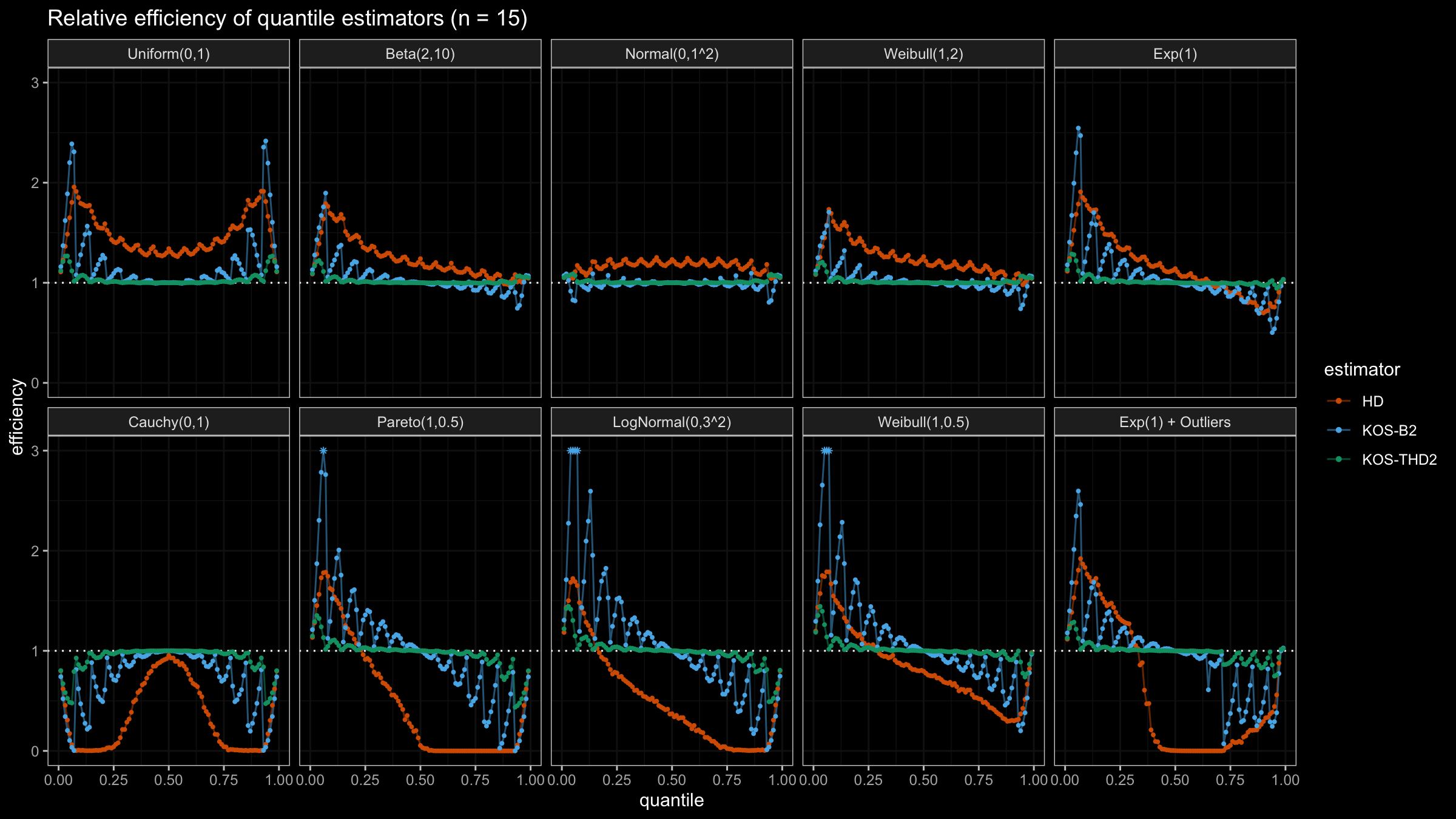
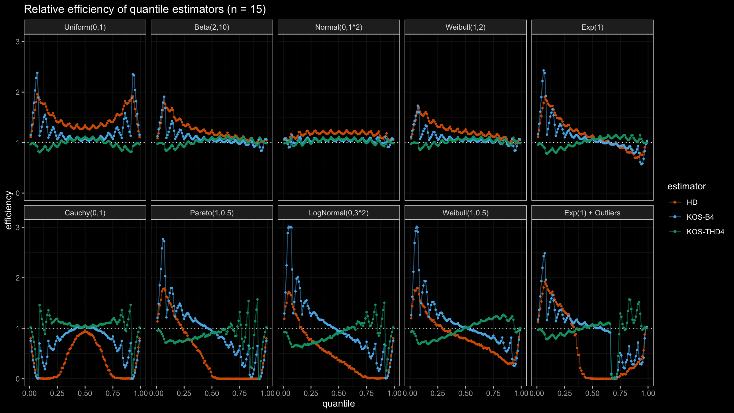
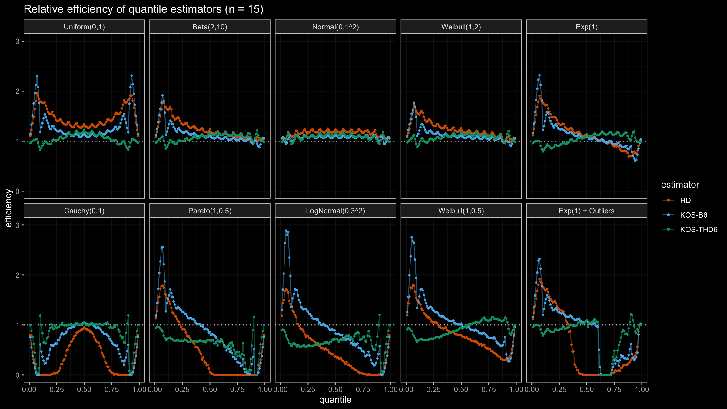
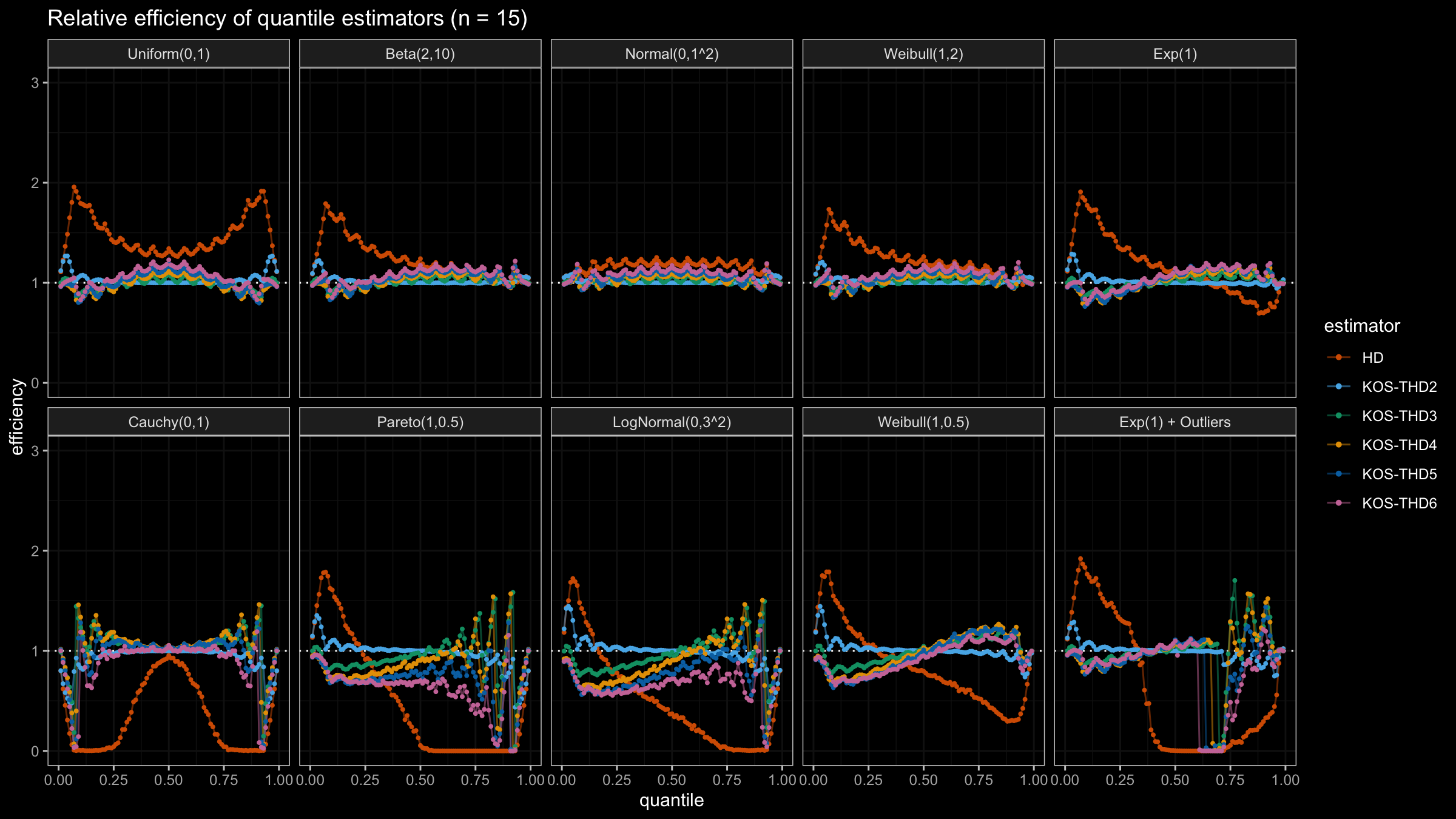
Here are some of the statistical efficiency plots:

Conclusion

The above plots are not so impressive: the suggested estimator has poor statistical efficiency. In the next post, we will try to make a few adjustments in order to solve this problem.