Quantile estimators based on k order statistics, Part 5: Improving trimmed Harrell-Davis quantile estimator

Andrey Akinshin · 2021-08-31

Update: this blog post is a part of research that aimed to build a statistically efficient and robust quantile estimator. A paper with final results is available in Communications in Statistics - Simulation and Computation (DOI: 10.1080/03610918.2022.2050396). A preprint is available on arXiv: arXiv:2111.11776 [stat.ME]. Some information in this blog post can be obsolete: please, use the official paper as the primary reference.

During the last several months, I have been experimenting with different variations of the trimmed Harrell-Davis quantile estimator. My original idea of using the highest density interval based on the fixed area percentage (e.g., HDI 95% or HDI 99%) led to a set of problems with overtrimming. I tried to solve them with manually customized trimming strategy, but this approach turned out to be too inconvenient; it was too hard to come up with optimal thresholds. One of the main problems was about the suboptimal number of elements that we actually aggregate to obtain the quantile estimation. So, I decided to try an approach that involves exactly k order statistics. The idea was so promising, but numerical simulations haven’t shown the appropriate efficiency level.

This bothered me the whole week. It sounded so reasonable to trim the Harrell-Davis quantile estimator using exactly k order statistics. Why didn’t this work as expected? Finally, I have found a fatal flaw in my previous approach: while it was a good idea to fix the size of the trimming window, I mistakenly chose its location following the equation from the Hyndman-Fan Type 7 quantile estimator!

In this post, we fix this problem and try another modification of the trimmed Harrell-Davis quantile estimator based on k order statistics and highest density intervals at the same time.

All posts from this series:

The problem

First of all, let’s see in detail what’s wrong with the approach from the previous blog post. To illustrate the problem, let’s consider the following setting:

$$ n = 10, \quad k = 3, \quad p = 0.175. $$

Now let’s see the order statistics weights for the classic Harrell-Davis quantile estimator (HD) and its trimmed modifications based on the trimming window derived from the Hyndman-Fan Type 7 quantile estimator (THD-HF7):

	HD	THD-HF7
W[1]	0.2867	0.0000
W[2]	0.3610	0.4340
W[3]	0.2163	0.4614
W[4]	0.0949	0.1046
W[5]	0.0318	0.0000
W[6]	0.0079	0.0000
W[7]	0.0013	0.0000
W[8]	0.0001	0.0000
W[9]	0.0000	0.0000
W[10]	0.0000	0.0000

The weights in the THD-HF7 column don’t look right. Let’s see why do we have such a situation. For the above settings, we have $L = 0.14$ and $R=0.34$. Thus, to obtain THD-HF7 weights from the HD weights, we should take 60% of W[2], 100% of W[3], 40% of W[4], and normalize the values. As a result, we have a strange situation: W[3] > W[2] (while we have the opposite situation in the HD case), W[1] = 0 (while it has a noticeable impact on the result in the HD case).

Due to these illogical weight assignments, the statistical efficiency of THD-HF7 is poor (which was shown in the previous post).

It’s time to fix the problem and try another approach.

The updated approach

As stated earlier, we keep the idea of using k order statistics. It means that the size of the trimming window is fixed:

$$ R_k - L_k = (k - 1) / n. $$

However, we are going to change the location of this window so as to get the highest density interval (HDI) of the Beta distribution.

Numerical simulations

It’s time to check our update approach!

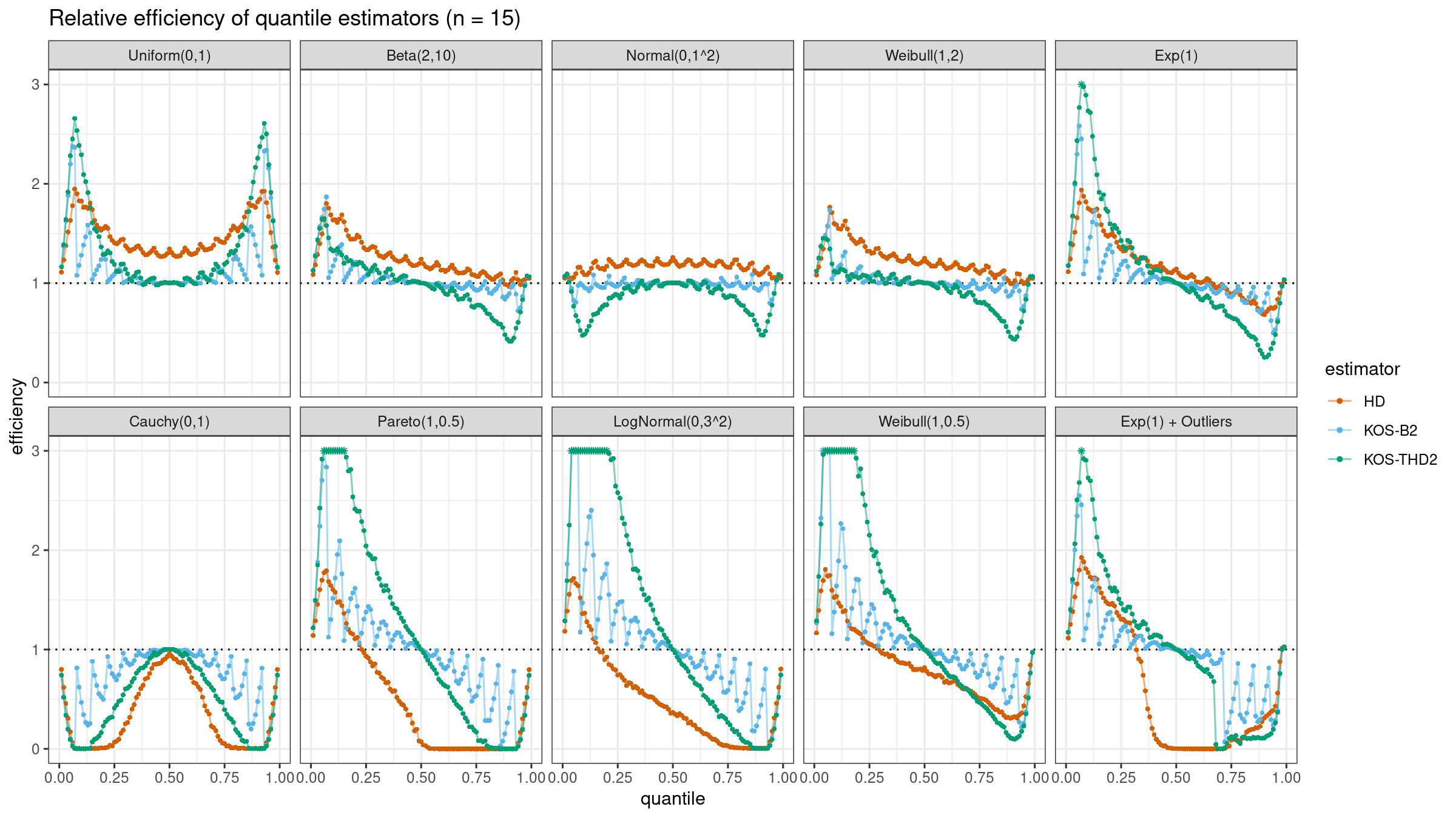
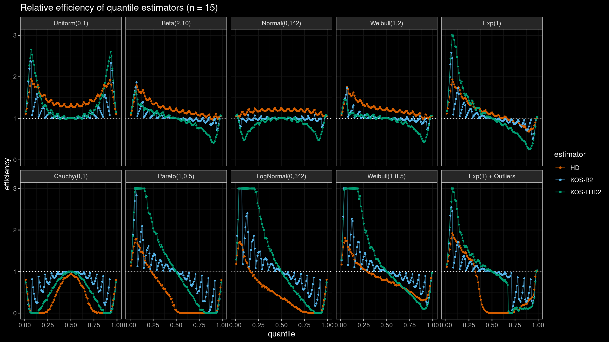
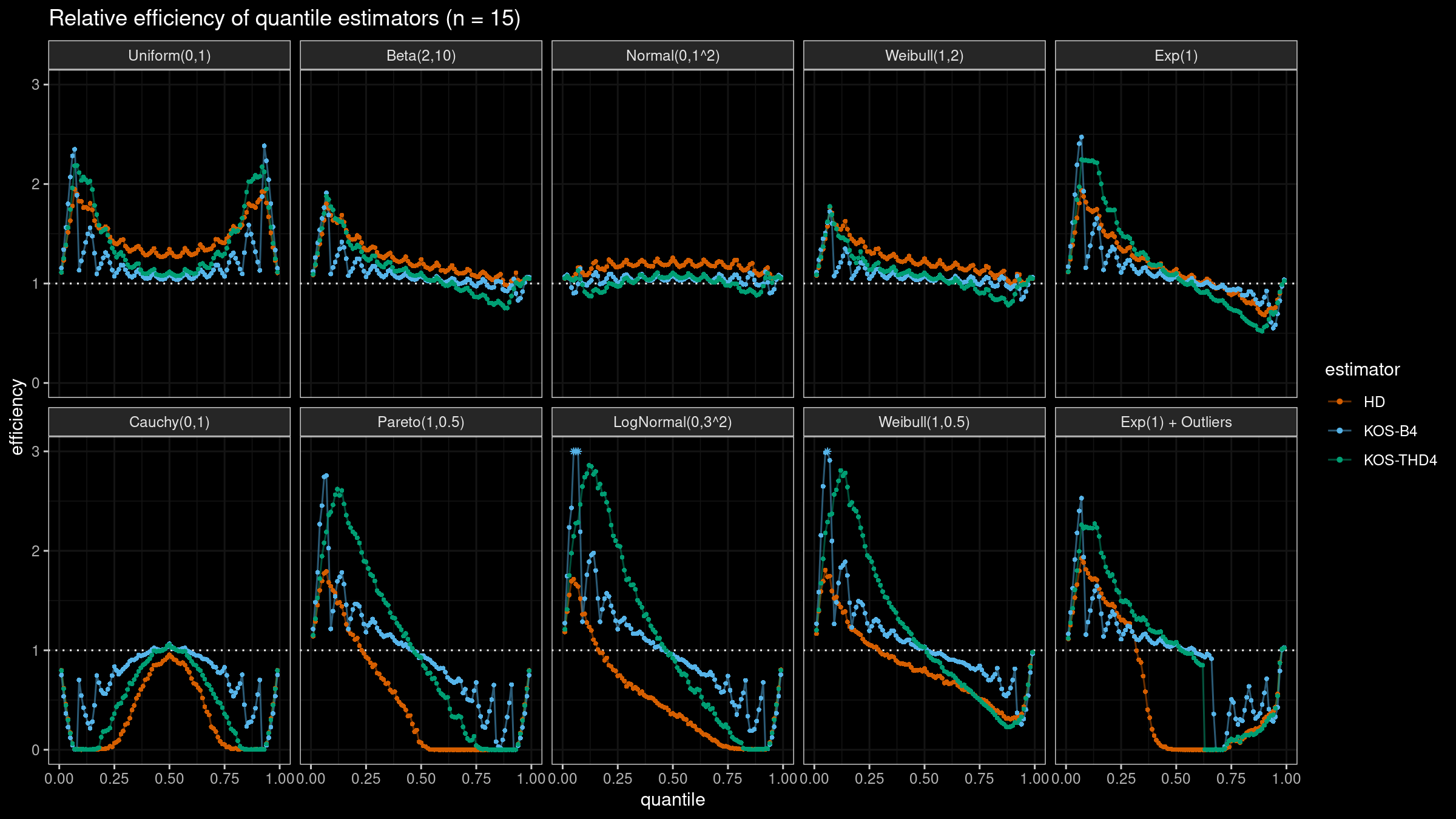
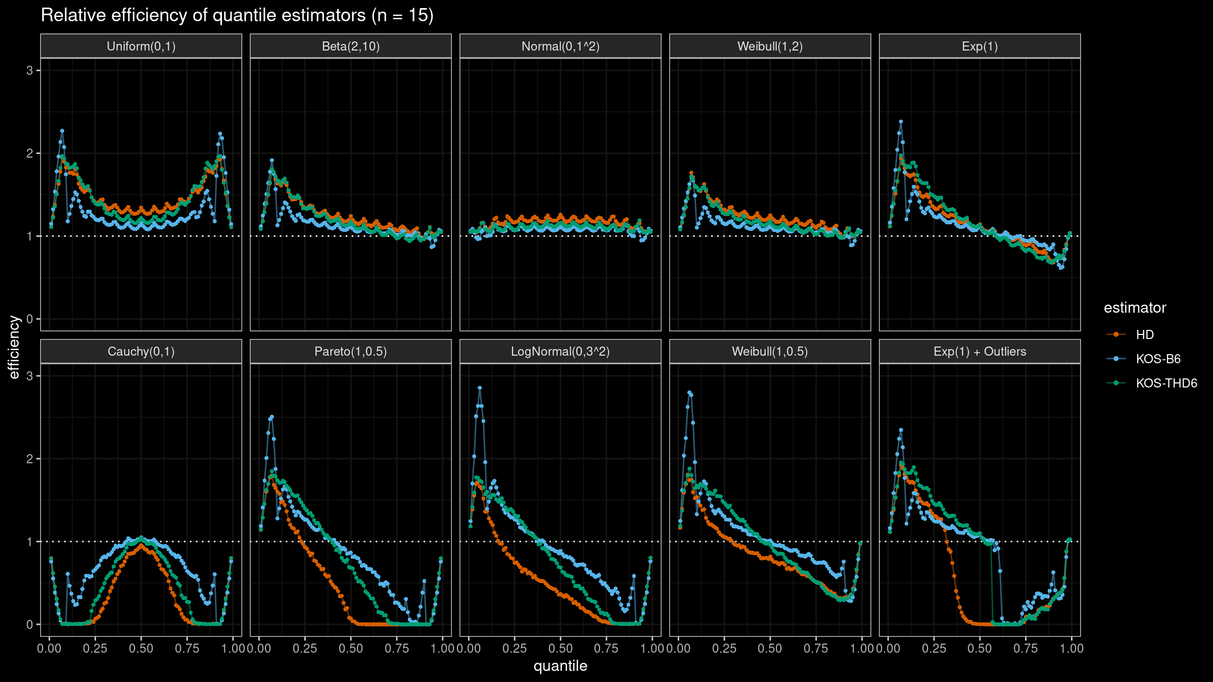
We are going to take the same simulation setup that was declared in this post. Briefly speaking, we evaluate the classic MSE-based relative statistical efficiency of different quantile estimators on samples from different light-tailed and heavy-tailed distributions using the classic Hyndman-Fan Type 7 quantile estimator as the baseline.

The considered estimator based on k order statistics is denoted as “KOS-THDk”. The estimator from the previous post based on the adjusted beta function is denoted as “KOS-Bk”.

Here are some of the statistical efficiency plots:

Conclusion

It sounds reasonable to use the trimmed modifications of the Harrell-Davis quantile estimator with the trimming strategy based on k order statistics. Unlike the originally proposed approach with the trimming strategy based on the highest density interval of the given area, the updated version of THD doesn’t become degenerated in the corner cases (the problem of over-trimming). Also, it provides more direct control of the estimator breakdown point, which is also a nice feature.

In the next post, I will try to come up with further improvements of the suggested estimator.