Quantile estimators based on k order statistics, Part 7: Optimal threshold for the trimmed Harrell-Davis quantile estimator

Andrey Akinshin · 2021-09-14

Update: this blog post is a part of research that aimed to build a statistically efficient and robust quantile estimator. A paper with final results is available in Communications in Statistics - Simulation and Computation (DOI: 10.1080/03610918.2022.2050396). A preprint is available on arXiv: arXiv:2111.11776 [stat.ME]. Some information in this blog post can be obsolete: please, use the official paper as the primary reference.

In the previous post, we have obtained a nice quantile estimator. To be specific, we considered a trimmed modification of the Harrell-Davis quantile estimator based on the highest density interval of the given size. The interval size is a parameter that controls the trade-off between statistical efficiency and robustness. While it’s nice to have the ability to control this trade-off, there is also a need for the default value, which could be used as a starting point when we have neither estimator breakdown point requirements nor prior knowledge about distribution properties.

After a series of unsuccessful attempts, it seems that I have found an acceptable solution. We should build the new estimator based on $\sqrt{n} / n$ order statistics. In this post, I’m going to briefly explain the idea behind the suggested estimator and share some numerical simulations that compare the proposed estimator and the classic Harrell-Davis quantile estimator.

All posts from this series:

The approach

The general idea is the same that was used in one of the previous posts. We express the estimation of the $p^{th}$ quantile as a weighted sum of all order statistics:

\begin{matrix} q_{p} = \sum_{i = 1}^{n} W_{i} \cdot x_{i}, \\ W_{i} = F (r_{i}) - F (l_{i}), \\ l_{i} = (i - 1) / n, r_{i} = i / n, \end{matrix}

where $F$ is a CDF function of a specific distribution. In the case of the Harrell-Davis quantile estimator, we use the Beta distribution. Thus, $F$ could be expressed via regularized incomplete beta function $I_{x} (α, β)$ :

F_{HD} (u) = I_{u} (α, β), α = (n + 1) p, β = (n + 1) (1 - p) .

In the case of the trimmed Harrell-Davis quantile estimator, we use only a part of the Beta distribution inside the $[L, R]$ window. Thus, $F$ could be expressed as rescaled regularized incomplete beta function inside the given window:

F_{THD} (u) = {\begin{array}{lcrcllr} 0 & for & u & < & L, \\ (F_{HD} (u) - F_{HD} (L)) / (F_{HD} (R) - F_{HD} (L)) & for & L & \leq & u & \leq & R, \\ 1 & for & R & < & u . \end{array}

In the previous post, we discussed the idea of choosing $L$ and $R$ as a highest density interval of the given width $R - L$ . In this post, we are going to express the window size via the sample size $n$ as follows:

R - L = \frac{\sqrt{n}}{n} .

If we don’t have any specific requirements for the estimator (e.g., the desired breakdown point) and we have no prior knowledge about distribution properties (e.g., the presence of a heavy tail), such an estimator looks like a good default option.

Numerical simulations

The relative efficiency value depends on five parameters:

Target quantile estimator
Baseline quantile estimator
Estimated quantile $p$
Sample size $n$
Distribution

As target quantile estimators, we use:

HD: Classic Harrell-Davis quantile estimator
THD-SQRT: The described above trimmed modification of the Harrell-Davis quantile estimator based on highest density interval of size $\sqrt{n} / n$ .

The conventional baseline quantile estimator in such simulations is the traditional quantile estimator that is defined as a linear combination of two subsequent order statistics. To be more specific, we are going to use the Type 7 quantile estimator from the Hyndman-Fan classification or HF7. It can be expressed as follows (assuming one-based indexing):

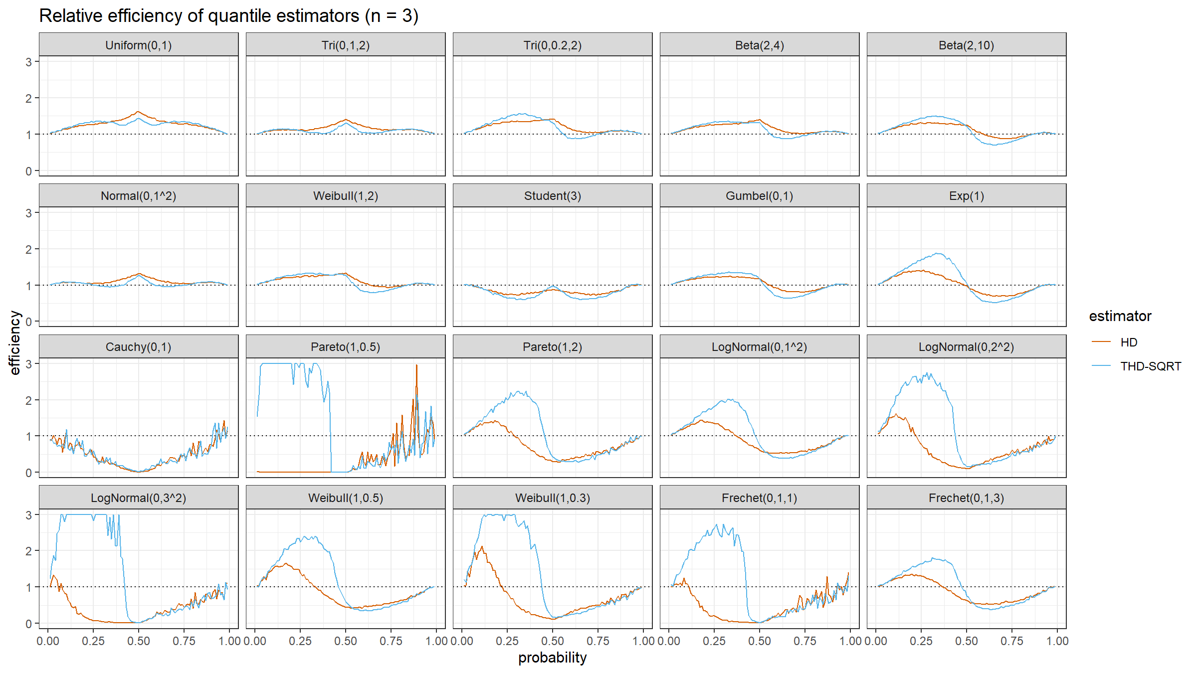
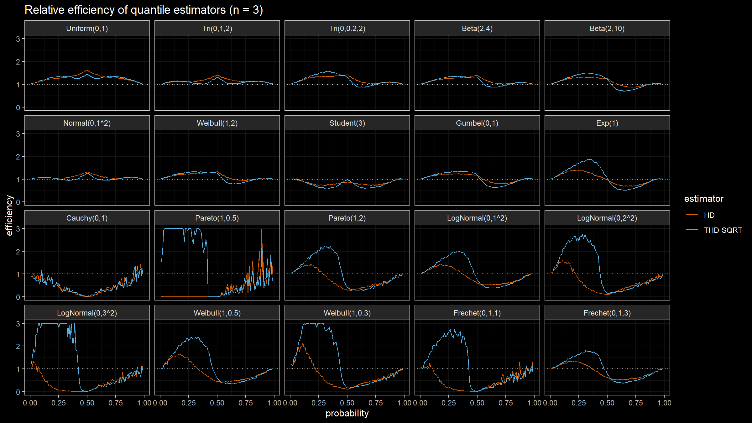
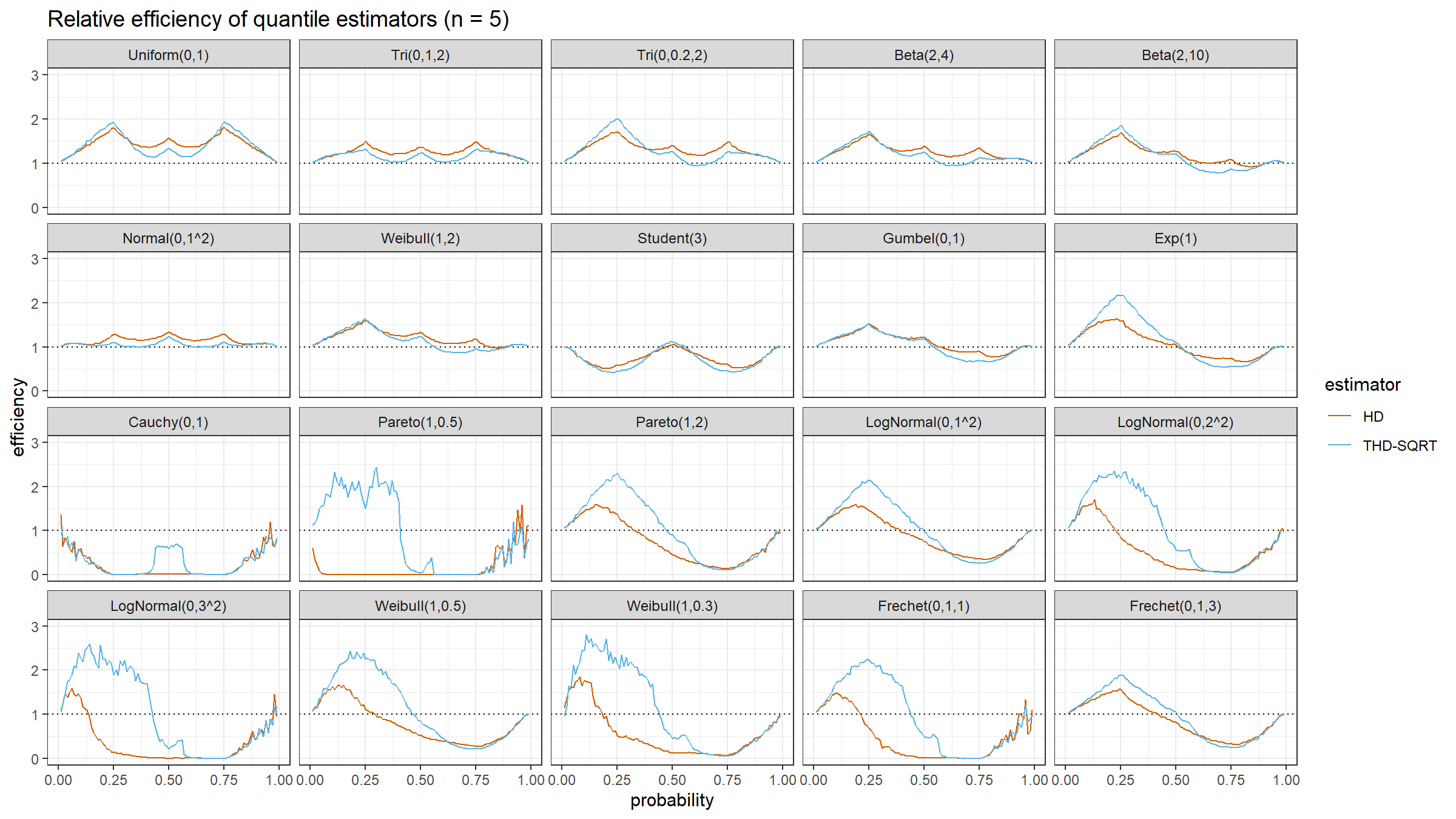
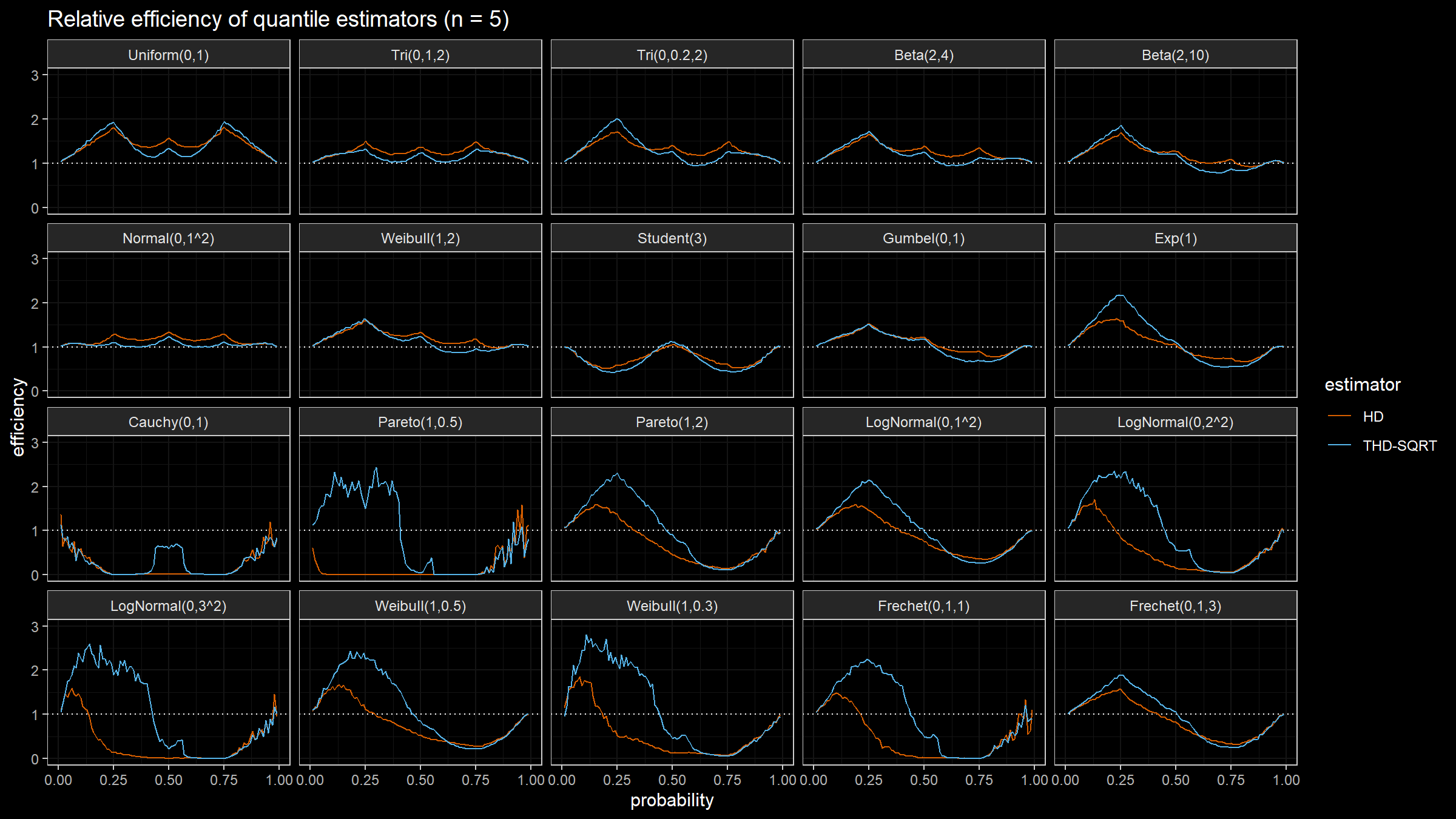
Q_{H F 7} (p) = x_{(⌊ h ⌋)} + (h - ⌊ h ⌋) (x_{(⌊ h ⌋ + 1)}) - x_{(⌊ h ⌋)}, h = (n - 1) p + 1.

Thus, we are going to estimate the relative efficiency of the trimmed Harrell-Davis quantile estimator with different percentage values against the traditional quantile estimator HF7. For the $p^{th}$ quantile, the classic relative efficiency can be calculated as the ratio of the estimator mean squared errors ( $MSE$ ):

Efficiency (p) = \frac{MSE (Q_{H F 7}, p)}{MSE (Q_{Target}, p)} = \frac{E [(Q_{H F 7} (p) - θ (p))^{2}]}{E [(Q_{Target} (p) - θ (p))^{2}]}

where $θ (p)$ is the true value of the $p^{th}$ quantile. The $MSE$ value depends on the sample size $n$ , so it should be calculated independently for each sample size value.

We are also going to use the following distributions:

Uniform(0,1): Continuous uniform distribution; $a = 0, b = 1$
Tri(0,1,2): Triangular distribution; $a = 0, c = 1, b = 2$
Tri(0,0.2,2): Triangular distribution; $a = 0, c = 0.2, b = 2$
Beta(2,4): Beta distribution; $α = 2, β = 4$
Beta(2,10): Beta distribution; $α = 2, β = 10$
Normal(0,1^2): Standard normal distribution; $μ = 0, σ = 1$
Weibull(1,2): Weibull distribution; $λ = 1 (scale), k = 2 (shape)$
Student(3): Student distribution; $ν = 3 (degrees of freedom)$
Gumbel(0,1): Gumbel distribution; $μ = 0 (location), β = 1 (scale)$
Exp(1): Exponential distribution; $λ = 1 (rate)$
Cauchy(0,1): Standard Cauchy distribution; $x_{0} = 0 (location), γ = 1 (scale)$
Pareto(1,0.5): Pareto distribution; $x_{m} = 1 (scale), α = 0.5 (shape)$
Pareto(1,2): Pareto distribution; $x_{m} = 1 (scale), α = 2 (shape)$
LogNormal(0,1^2): Log-normal distribution; $μ = 0, σ = 1$
LogNormal(0,2^2): Log-normal distribution; $μ = 0, σ = 2$
LogNormal(0,3^2): Log-normal distribution; $μ = 0, σ = 3$
Weibull(1,0.5): Weibull distribution; $λ = 1 (scale), k = 0.5 (shape)$
Weibull(1,0.3): Weibull distribution; $λ = 1 (scale), k = 0.3 (shape)$
Frechet(0,1,1): Frechet distribution; $m = 0 (location), s = 1 (scale), α = 1 (shape)$
Frechet(0,1,3): Frechet distribution; $m = 0 (location), s = 1 (scale), α = 3 (shape)$

Simulation Results

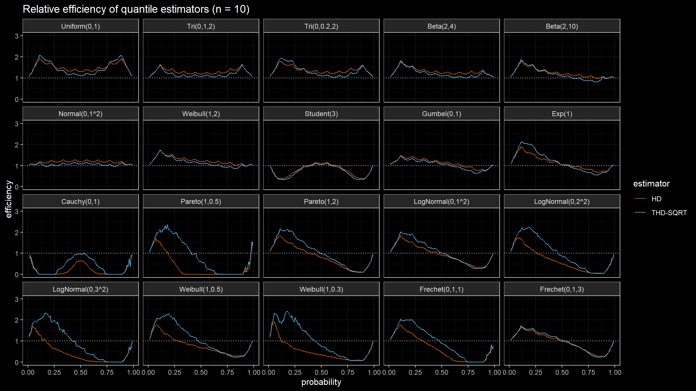
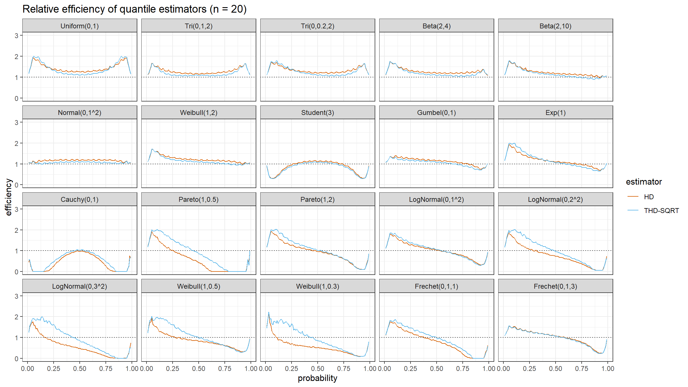
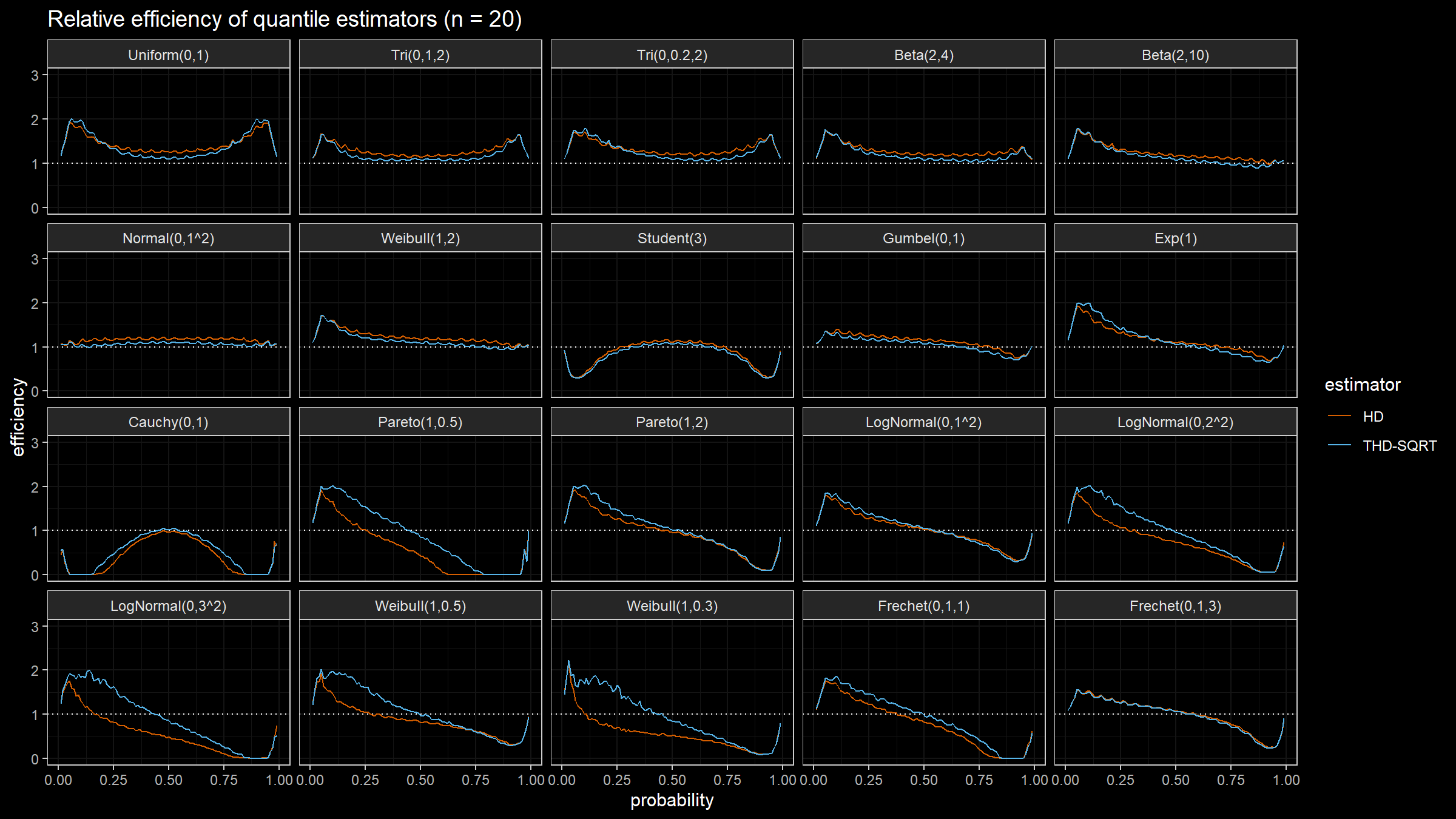
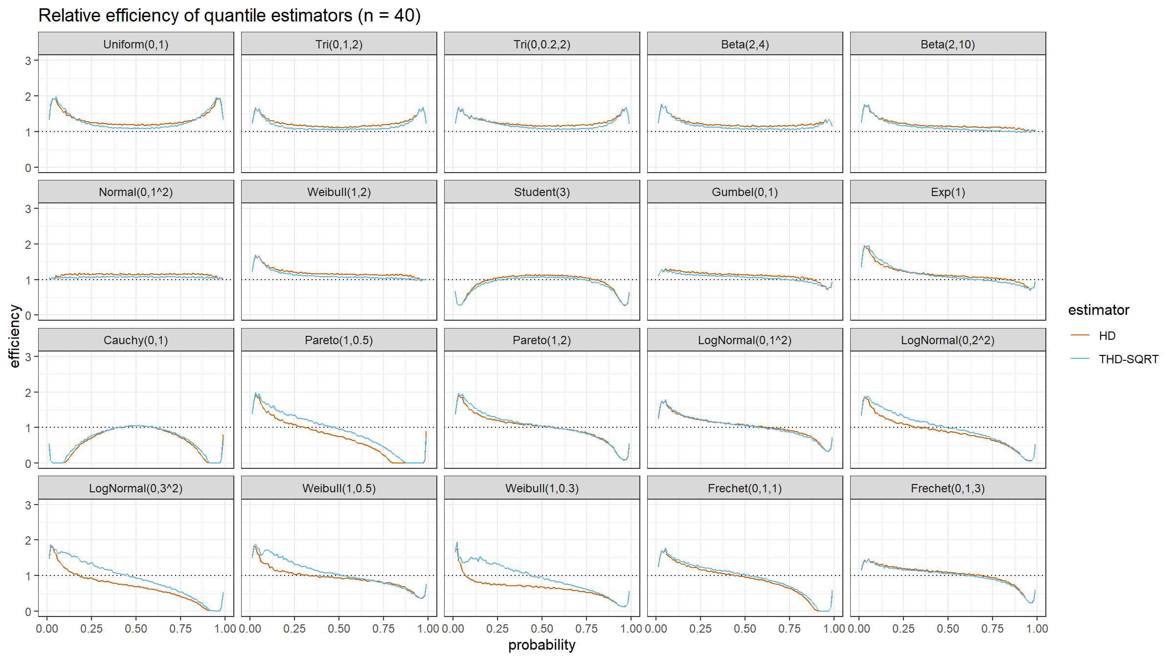
Conclusion

The trimmed modification of the Harrell-Davis quantile estimator based on the highest density interval of size $\sqrt{n} / n$ looks like a good option for a “default” quantile estimator for different applications. In the next blog posts, we will continue to evaluate different options of the suggested approach.