Caveats of using the median absolute deviation
The below text contains an intermediate snapshot of the research and is preserved for historical purposes.
The median absolute deviation is a measure of dispersion which can be used as a robust alternative to the standard deviation. It works great for slight deviations from normality (e.g., for contaminated normal distributions or slightly skewed unimodal distributions). Unfortunately, if we apply it to distributions with huge deviations from normality, we may experience a lot of troubles. In this post, I discuss some of the most important caveats which we should keep in mind if we use the median absolute deviation.
Introduction
Let $X$ be a sample of i.i.d. random variables: $X = \{ X_1, X_2, \ldots, X_n \}$. The median absolute deviation is defined as follows
$$ \operatorname{MAD}(X) = C \cdot \operatorname{median}(|X - \operatorname{median}(X)|), $$where $C$ is the scale constant, $\operatorname{median}$ is the median estimator. In the scope of this post, we use only the classic sample median (if $n$ is odd, the median is the middle order statistic; if $n$ is even, the median is the arithmetic average of the two middle order statistics). The scale constant $C$ allows using $\operatorname{MAD}$ as a consistent estimator of the standard deviation. In order to make $\operatorname{MAD}$ asymptotically consistent with the standard deviation under normality, we should use $C = 1 / \Phi^{-1}(0.75) \approx 1.4826$. In practice, we may need adjusted values of $C$ for small samples to obtain an unbiased estimator.
Using $\operatorname{MAD}$ as a robust replacement for the standard deviation may be reasonable in the case of slight deviations from normality. However, it could be quite misleading in the case of large deviations. Let us review some of the typical assumptions that may lead to incorrect conclusions.
Caveat 1: Beware of the narrow estimation range assumption
With non-robust estimators, a single corrupted element can easily distort the estimation. A transition towards robust approaches brings a lot of benefits in terms of stability: a single altered element cannot introduce extreme changes in the estimation value. Having this knowledge, many researchers typically expect that robust estimations would fit a narrow range of values. Therefore, they can omit the phase of exploring the distribution of estimations and draw conclusions based on a single trial assuming that all possible estimations are close enough to each other. However, while robust estimators indeed provide a decent defense against extreme outliers, they still can have a wide range of possible values.
Let us consider an example. In the below figure, we can see a density plot of a trimodal distribution.
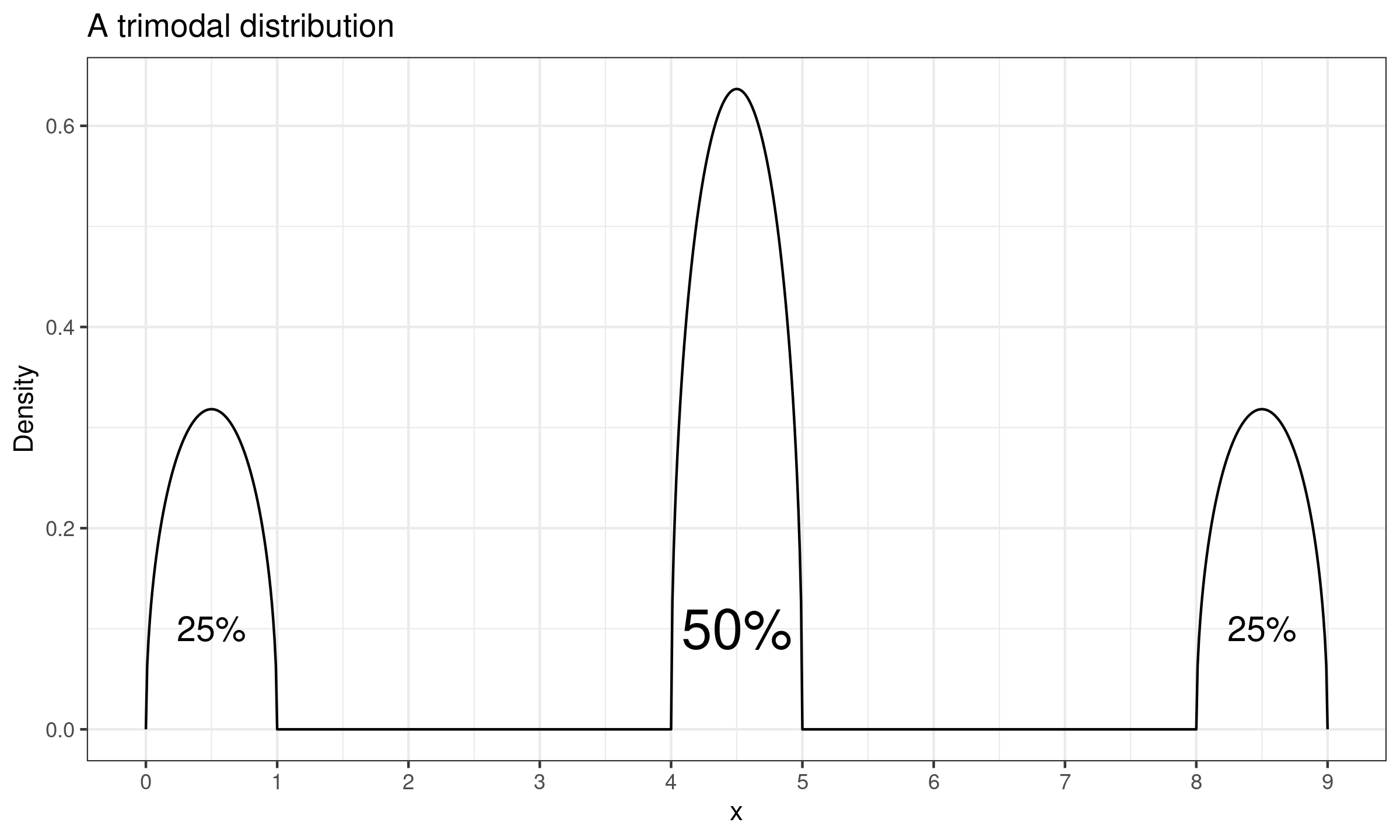
This distribution has three non-intersecting intervals: $[0;1]$ ($25\%$ of the distribution), $[4;5]$ ($50\%$ of the distribution), and $[8;9]$ ($25\%$ of the distribution). While the distribution has an unambiguously defined median $M = 4.5$, its quantile function of the absolute deviations around the median ($|X - \operatorname{median}(X)|$) has a discontinuity at 0.5. This means unambiguously define the $\operatorname{MAD}$ value. Indeed, the $[M-\operatorname{MAD}; M+\operatorname{MAD}]$ interval should cover exactly $50\%$ of the distribution. In the considered case, there are multiple ways to define such an interval. The interval value various from $[4;5]$ to $[1;8]$.
Now we explore practical implications of working with such a distribution. Let us take $1\,000$ random samples of size $100$ from this distribution, estimate the $\operatorname{MAD}$ value for each sample, and build a new distribution based on the obtained estimations. The density plot of the observed sampling distribution is presented in the below figure (we use the kernel density estimation with the normal kernel and the Sheather & Jones method to select the bandwidth).
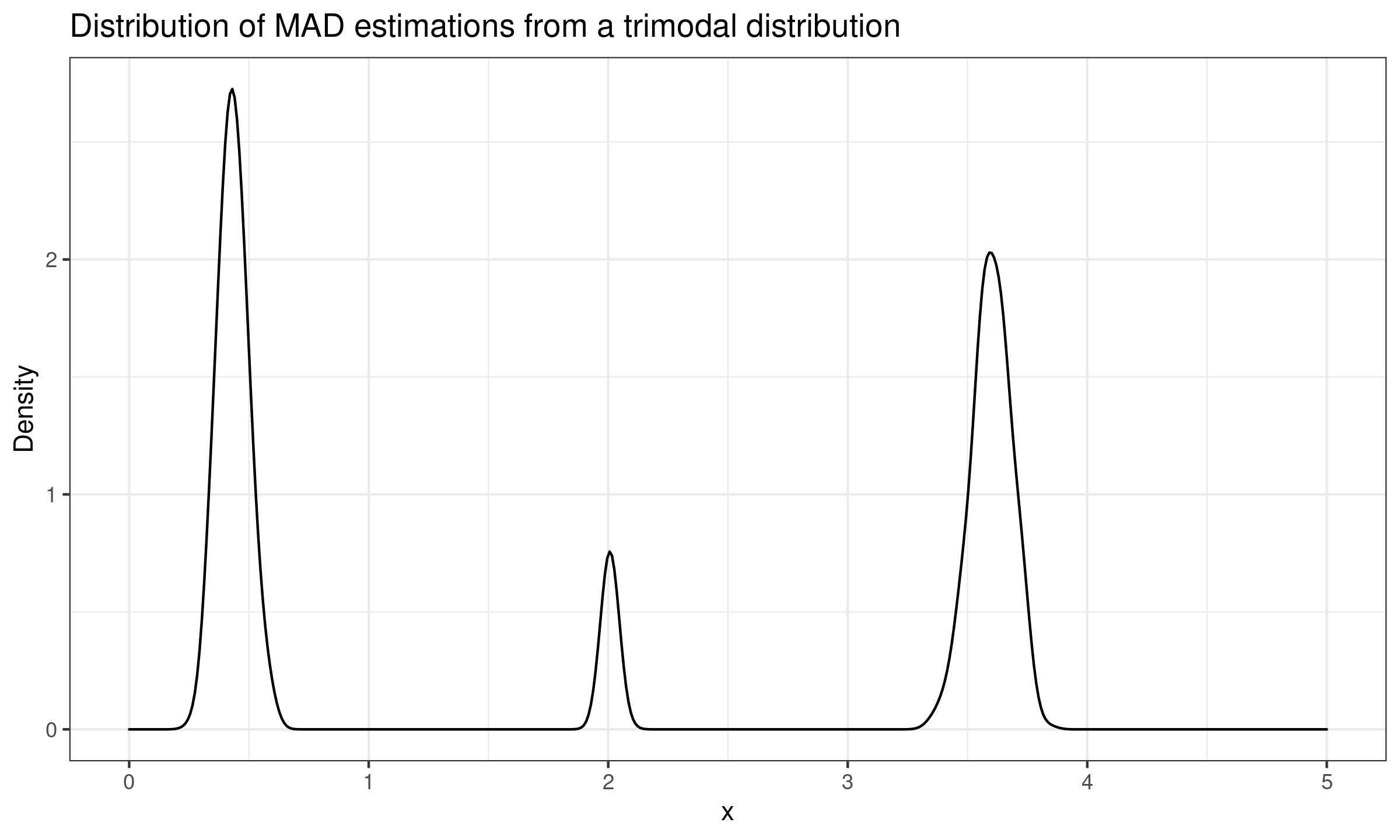
As we can see, the sampling $\operatorname{MAD}$ distribution is also trimodal. In the general case, the distance between these modes could be as large as a gap around the $0.5^\textrm{th}$ quantile of $|X - \operatorname{median}(X)|$.
Thus, if the original distribution is not unimodal, we cannot speculate on the form of the sampling $\operatorname{MAD}$ distribution based just on a few of the $\operatorname{MAD}$ estimations.
Caveat 2: Beware of the non-zero dispersion assumption
Another popular assumption about the measures of dispersion is that they always positive. It is almost true for the standard deviation: unless all sample elements are equal to each other, the standard deviation is always positive. Thanks to this property, the standard deviation is often used as a denominator in various statistical equations (e.g., in effect size measures like the Cohen’s d or null hypothesis significance tests like the Student’s t-test). In most cases, we shouldn’t expect division by zero because it’s almost impossible to get a sample taken from a continuous distribution in which all the elements are equal. Unfortunately, when we switch to robust measures of dispersion of non-parametric distributions, the risk of getting zero dispersion increases. We should be ready to get zero dispersion when we work with discrete distributions or mixtures of discrete and continuous distributions.
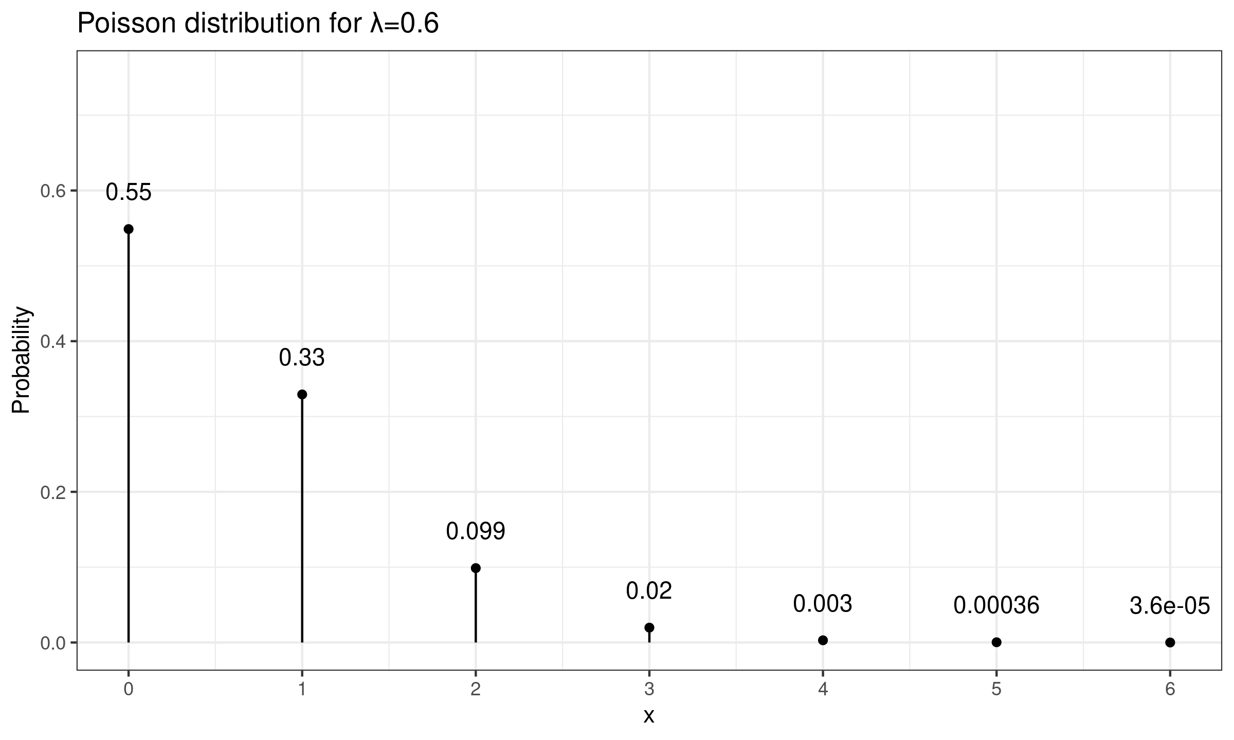
As an example of a discrete distribution, let us consider the Poisson distribution $\operatorname{Pois}(\lambda)$. Its probability mass function is defined as $p(k)=\lambda^k e^{-\lambda} / k!$. It’s easy to see that when $\lambda < \lambda_0 = -\ln(0.5) \approx 0.6931$, $p(0) > 0.5$. In this case, more than half of the distribution elements are equal to zero. Therefore, the median absolute deviation also becomes zero. In the below figure, a probability mass function of $\operatorname{Pois}(0.6)$ is presented. We can see that $p(0) \approx 0.55$ which gives us zero $\operatorname{MAD}$.
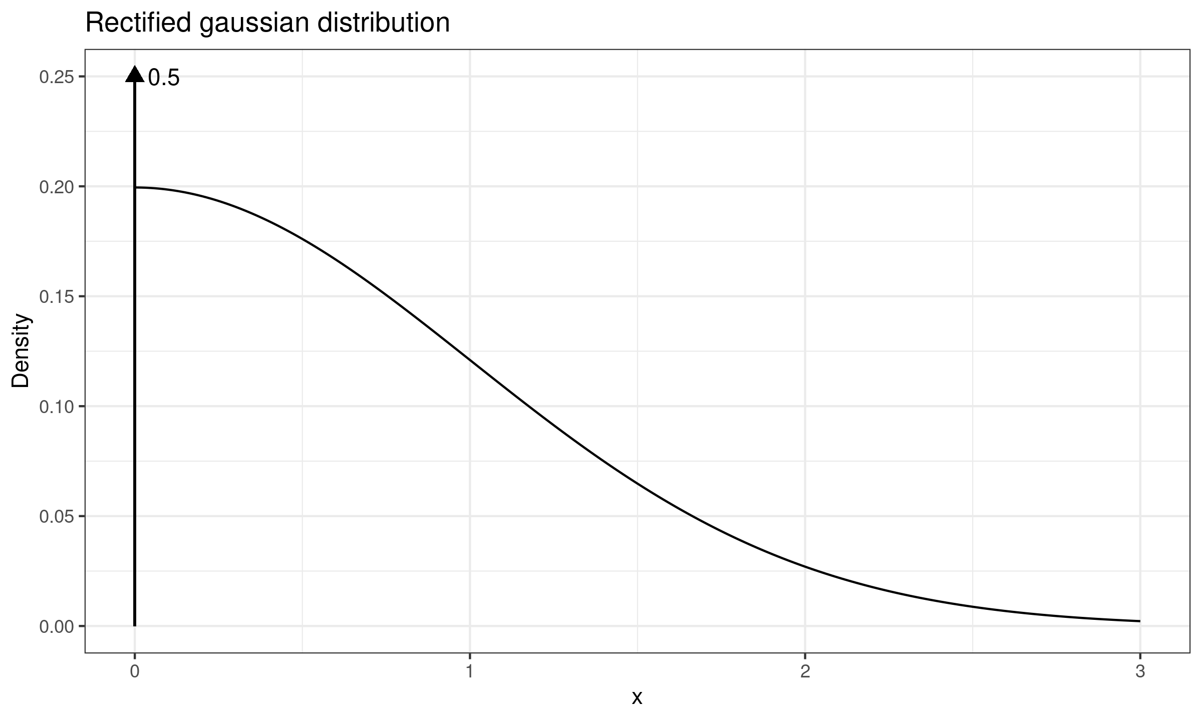
As an example of a mixture of discrete and continuous distributions, we can consider the rectified Gaussian distribution (presented in the below figure). It is a modification of the normal distribution in which all negative elements are replaced by zeros. It can be also represented as a mixture of the Dirac delta function $\delta(0)$ and the positive part of the normal distribution. Since $\delta(0)$ occupies exactly $50\%$ of the distribution, its median absolute deviation is also zero.
Distributions with zero $\operatorname{MAD}$ often arise in various disciplines. Since they are obviously non-normal, they require robust non-parametric analysis approach. However, the median absolute deviation is not always a good choice. For example, it doesn’t allow comparing dispersion estimations of two rectified Gaussian distributions or two Poisson distributions with $\lambda < 0.6931$. A blind usage of $\operatorname{MAD}$ as a denominator in automated statistical analysis can lead to a critical failure of the system.
Caveat 3: Beware of the 68–95–99.7 assumption
In the previous sections, we have reviewed multimodal distributions and discrete distributions. Once such features of the distributions are discovered, it becomes obvious that we cannot use classic assumptions that are valid for the normal distribution. Now we consider a case of an unimodal continuous distribution. With distributions, researchers often tend to use the normal distribution as a mental model. In the below figure, the normal distribution density plot is presented.

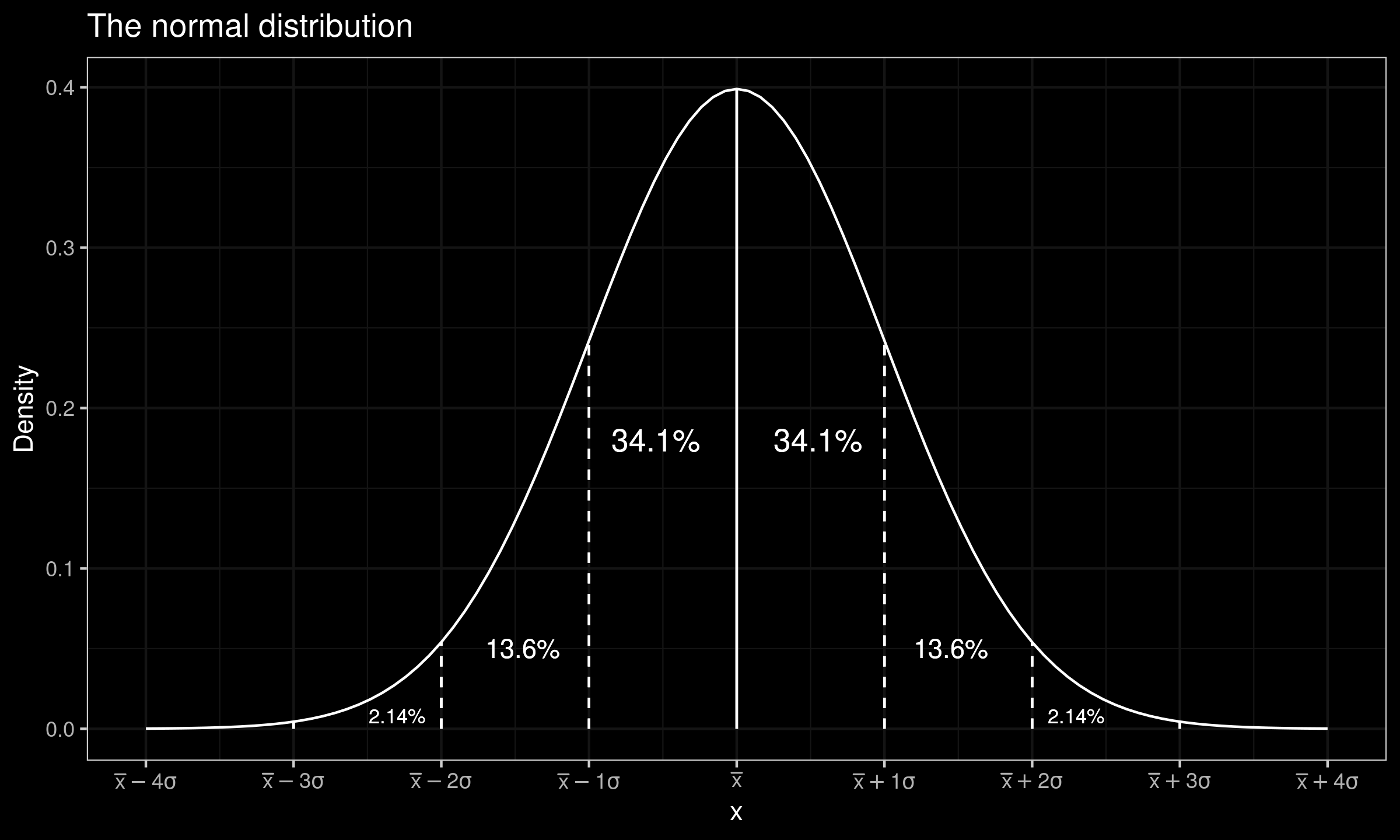
A typical assumption about the normal distribution is the 68–95–99.7 rule. It says that intervals $[\mu-\sigma;\mu+\sigma]$, $[\mu-2\sigma;\mu+2\sigma]$, and $[\mu-3\sigma;\mu+3\sigma]$ cover $68\%$, $95\%$, and $99.7\%$ of the normal distribution respectively. This rule is linked with the three-sigma rule of thumb that implies that the interval $[\mu-3\sigma;\mu+3\sigma]$ covers $99.7\%$ of the distribution values. While this empirical rule is applicable to many unimodal continuous light-tailed distributions, it can be violated in the case of heavy-tailed distributions.
Let us consider the Fréchet distribution with shape equals $1$, scale equals $1$, location equals $0$. It is a commonly used example of heavy-tailed distribution. Its true median value is $M \approx 1.44$ and the true median absolute deviation values is $\operatorname{MAD} \approx 0.9$. Its density plot is presented in the below figure:
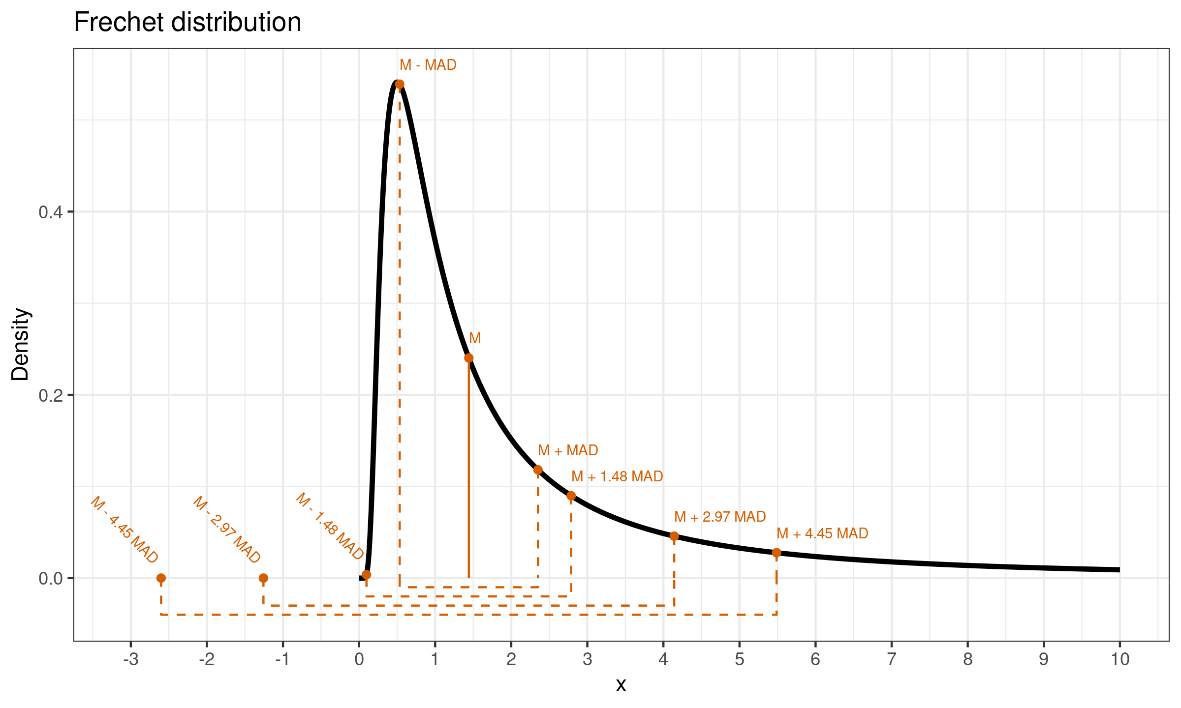
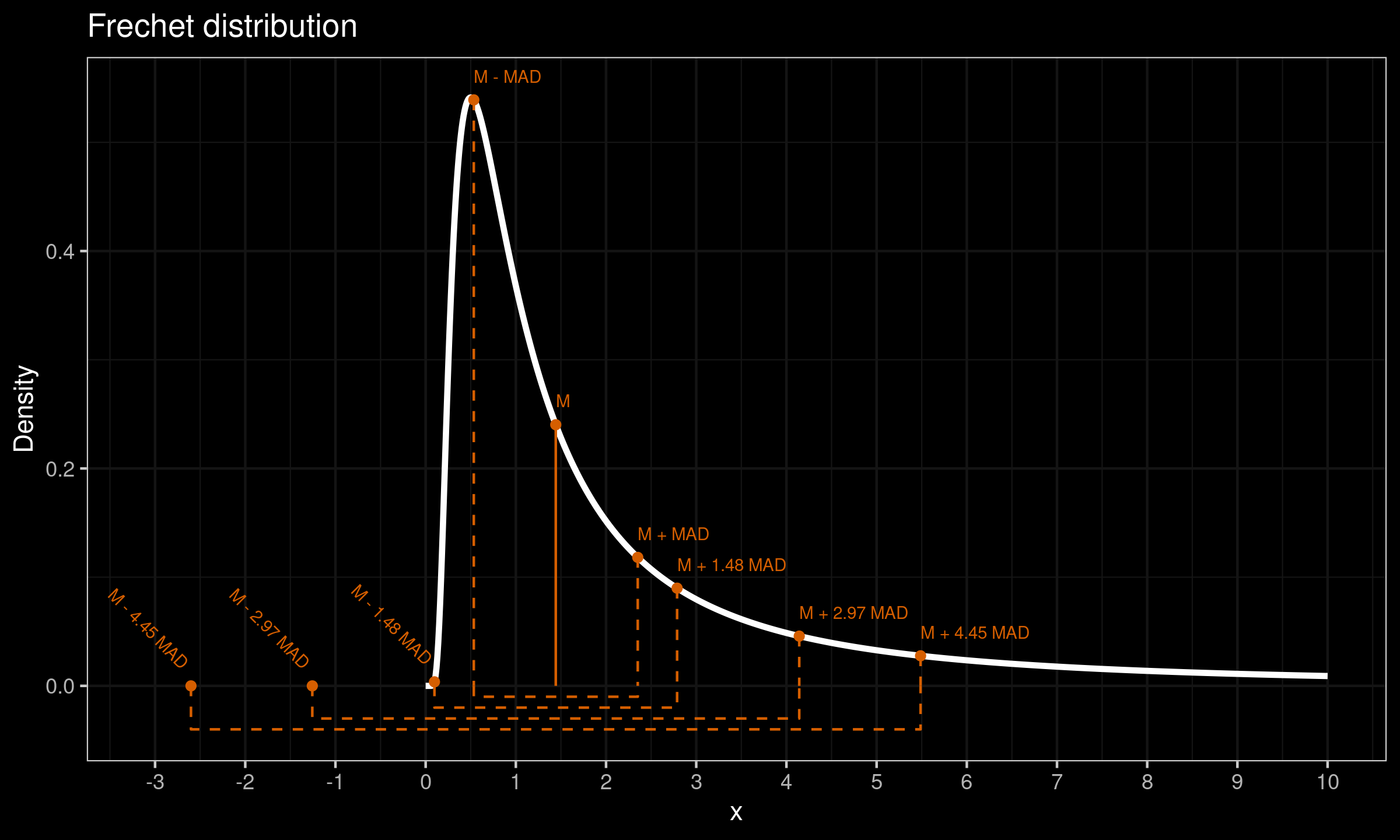
The variance of this distribution is infinite, therefore we can’t use the standard deviation as a measure of dispersion. However, we will check what would happen with the three-sigma rule if we try to apply it using a scaled $\operatorname{MAD}$ as a standard deviation estimator. Using the conventional value $C = 1.4826$, we get $C\cdot \mathrm{MAD} \approx 2.14$. Now let us consider intervals $[M-k \cdot \mathrm{MAD}; M+k \cdot \mathrm{MAD}]$ for $k \in \{ 1, C, 2C, 3C \}$. The actual coverage of each interval is presented in the following table:
| $k$ | $\mathbb{P}(M - k\cdot \mathrm{MAD} \leq X \leq \mathbb{P}(M + k\cdot \mathrm{MAD})$ |
|---|---|
| 1.00 | 0.500 |
| 1.48 | 0.699 |
| 2.97 | 0.786 |
| 4.45 | 0.833 |
As we can see, a blind usage of the three-sigma rule in the heavy-tailed case can lead to misleading insights. In the above example, the interval $[M- 3C \cdot \mathrm{MAD}; M+ 3C \cdot \mathrm{MAD}]$ actually cover only $83.3\%$ of the distribution instead of the typical $99.7\%$.
Conclusion
If we use a scaled median absolute deviation as a robust replacement to the standard deviation, we should be careful. It can work in an acceptable way for some unimodal continuous light-tailed distributions. However, distribution features like multimodality, discretization, or heavy-tailedness can easily violate our typical assumptions that we use with the normal distribution and the standard deviation.