Estimating quantile confidence intervals: Maritz-Jarrett vs. jackknife

When it comes to estimating quantiles of the given sample, my estimator of choice is the Harrell-Davis quantile estimator (to be more specific, its trimmed version). If I need to get a confidence interval for the obtained quantiles, I use the Maritz-Jarrett method because it provides a decent coverage percentage. Both approaches work pretty nicely together.

However, in the original paper by Harrell and Davis (1982), the authors suggest using the jackknife variance estimator in order to get the confidence intervals. The obvious question here is which approach better: the Maritz-Jarrett method or the jackknife estimator? In this post, I perform a numerical simulation that compares both techniques using different distributions.

Numerical simulation

Let’s consider a set of different distributions that includes symmetric/right-skewed and light-tailed/heavy-tailed options:

• beta(2,10): the Beta distribution (a = 2, b = 10)
• cauchy: the standard Cauchy distribution (location = 0, scale = 1)
• gumbel: the Gumbel distribution
• log-norm(0,3): the Log-normal distribution ($\mu$ = 0, $\sigma$ = 3)
• pareto(1,0.5): the Pareto distribution ($x_m$ = 1, $\alpha$ = 0.5)
• weibull(1,2): the Weibull distribution ($\lambda$ = 1, $k$ = 2) (light-tailed)
• uniform(0,1): the uniform distribution (a=0, b=1)
• normal(0,1): the standard normal distribution ($\mu$ = 0, $\sigma$ = 1)

For each distribution, we choose the evaluated quantile (P25, P50, P75, P90), the confidence level (0.90, 0.95, 0.99), and the sample size (3..50). Next, we generate a random sample 1000 times, evaluate the target confidence interval the Maritz-Jarrett method and the jackknife estimator, and check if we cover the true quantile value or not using for each approach.

Median

First of all, let’s look at the confidence interval estimations around the median.

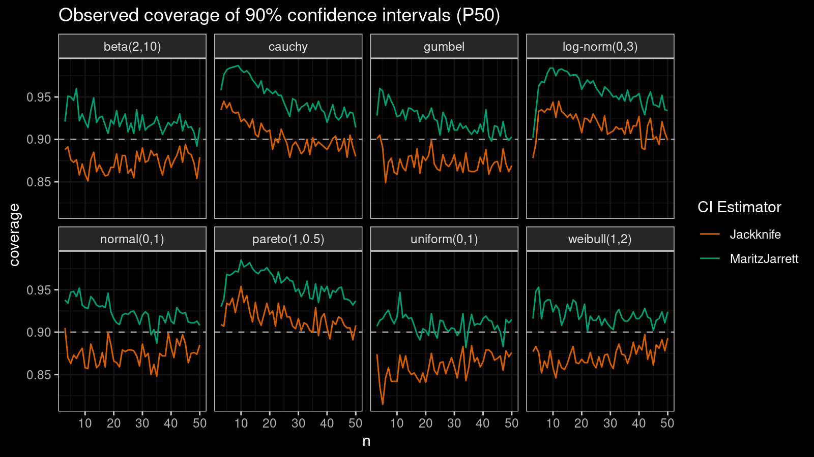
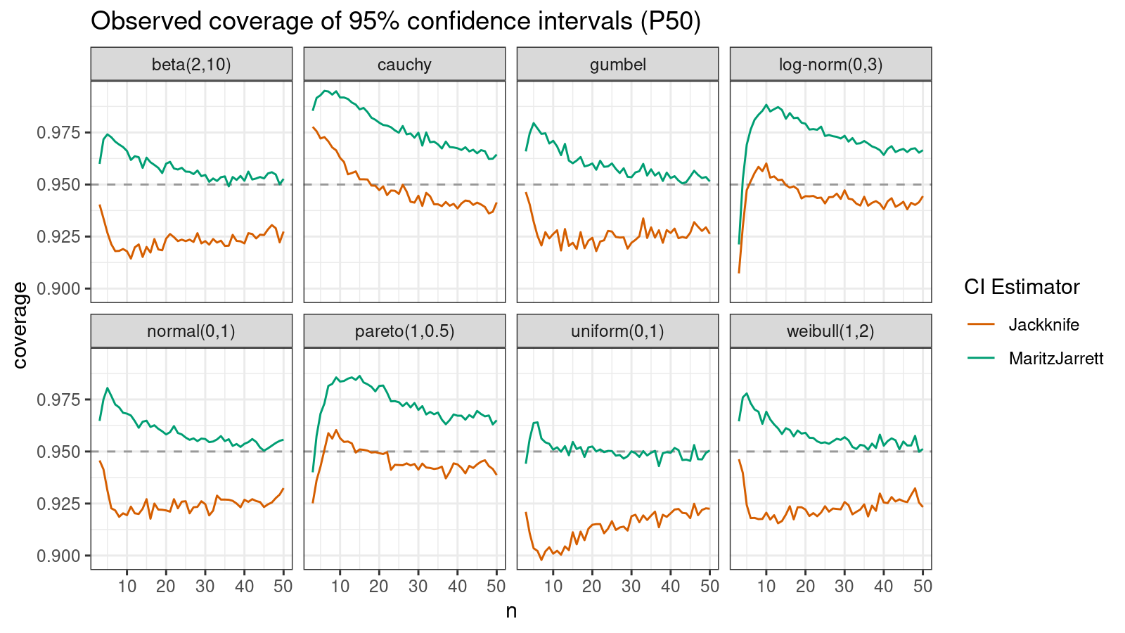
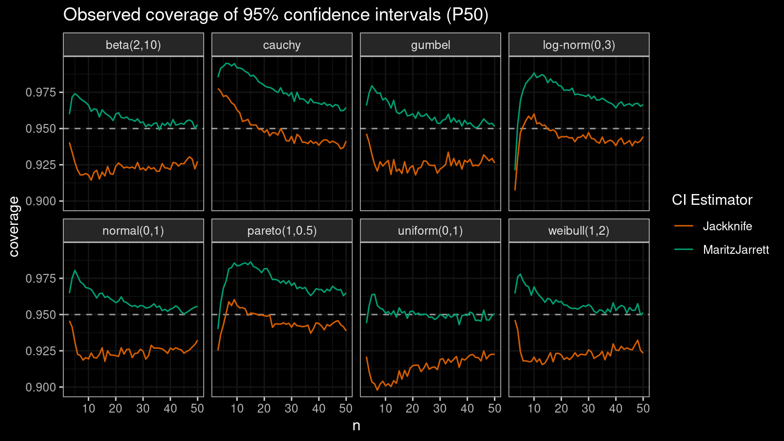
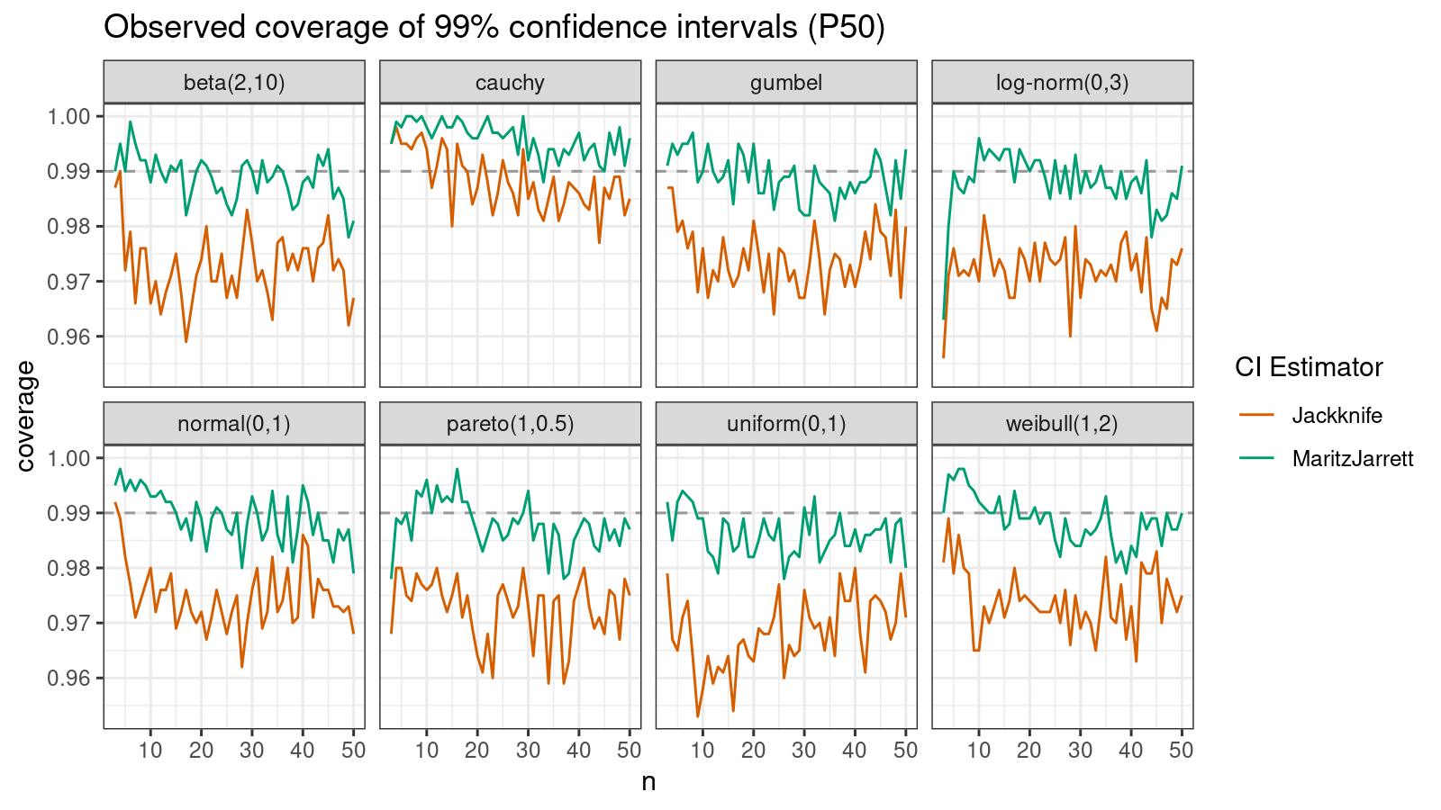
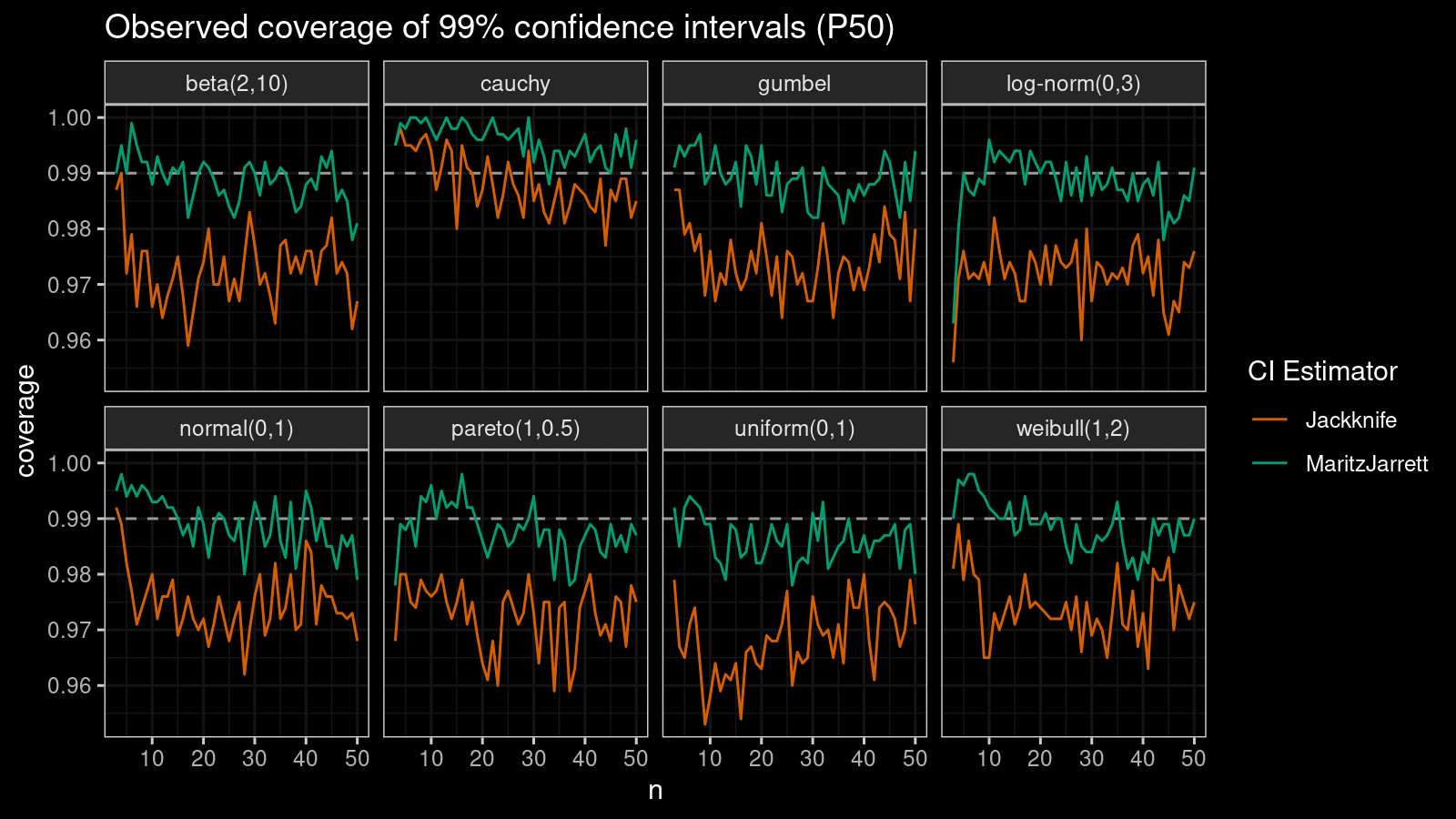
As we can see, the Maritz-Jarrett method produces better coverage values in all cases.

P25

Now let’s check the $25^\textrm{th}$ percentile.

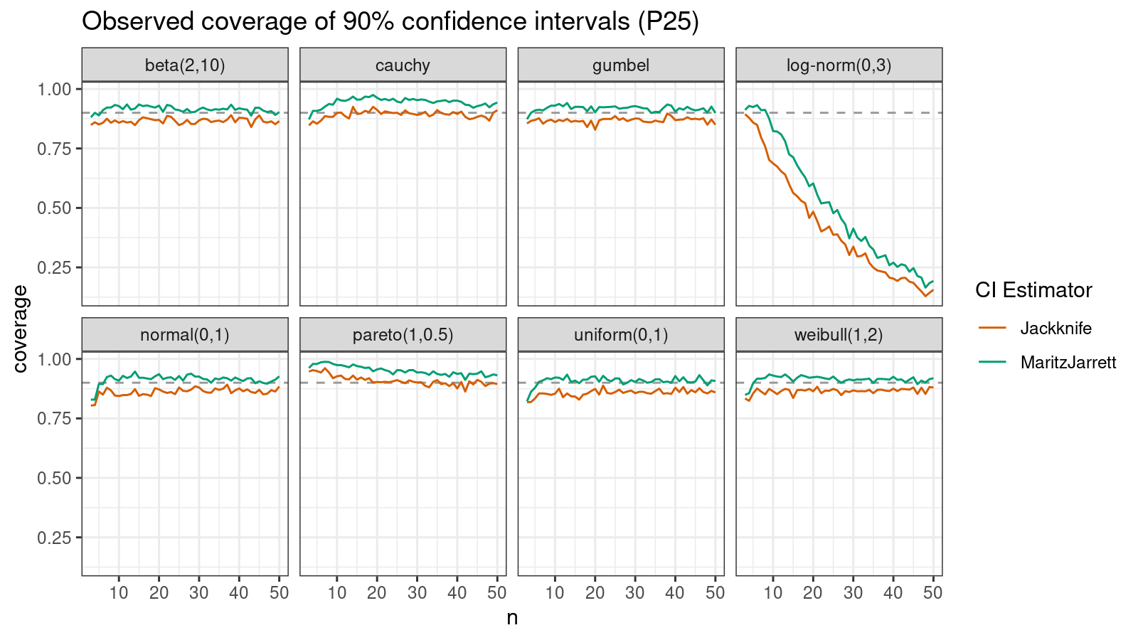
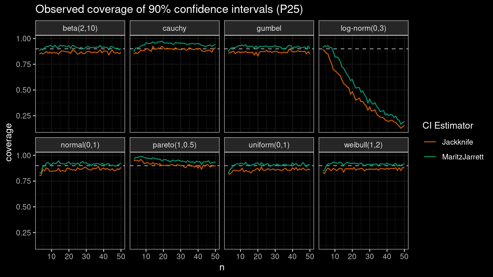
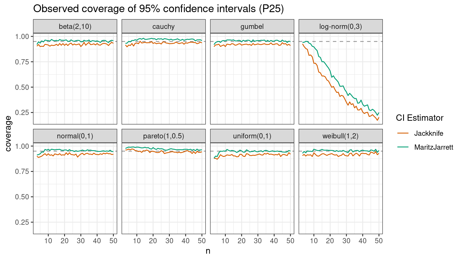
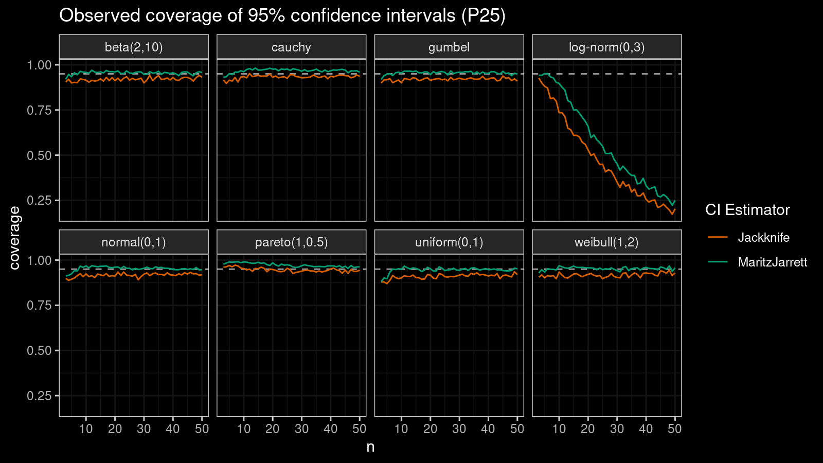
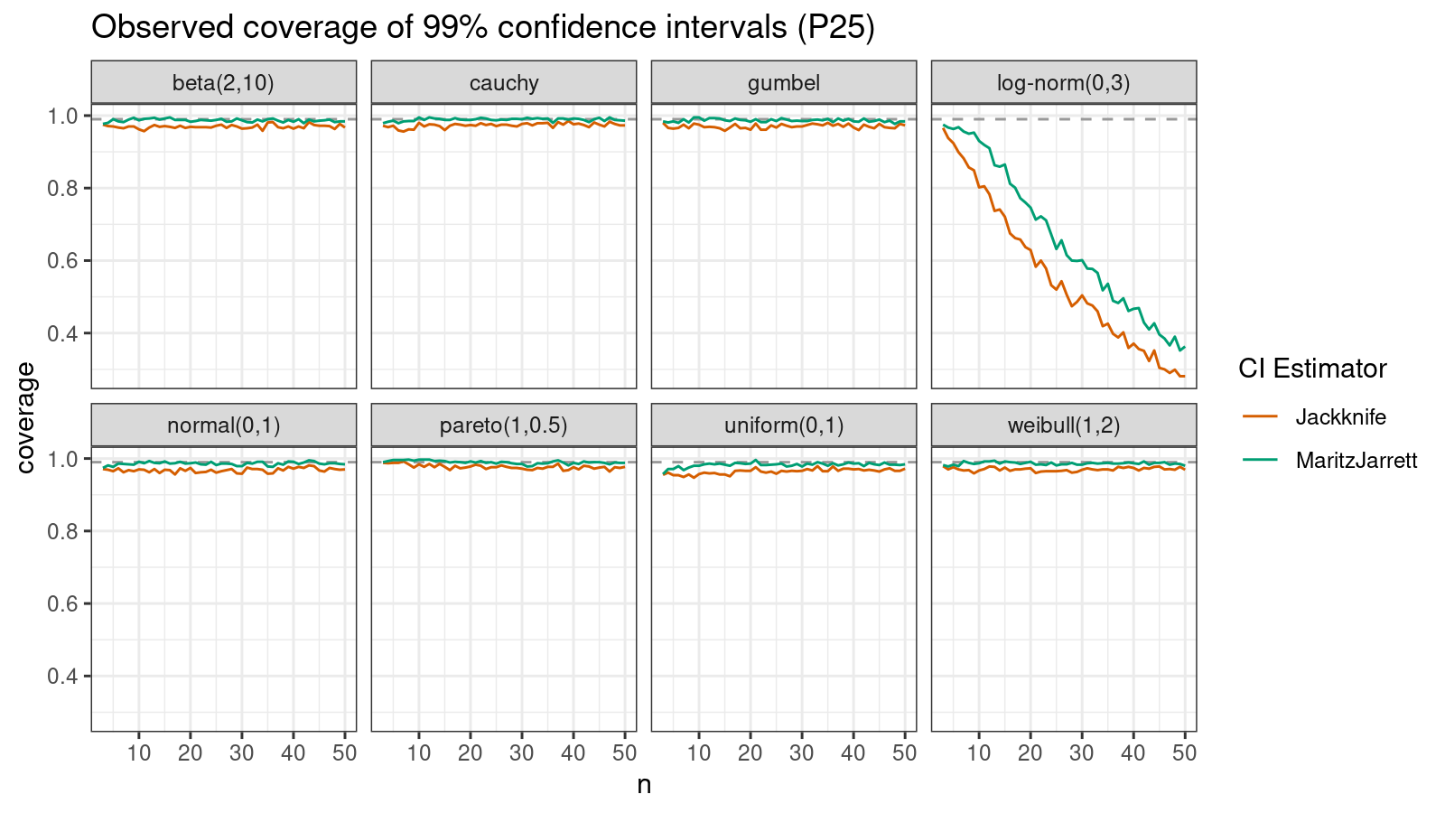
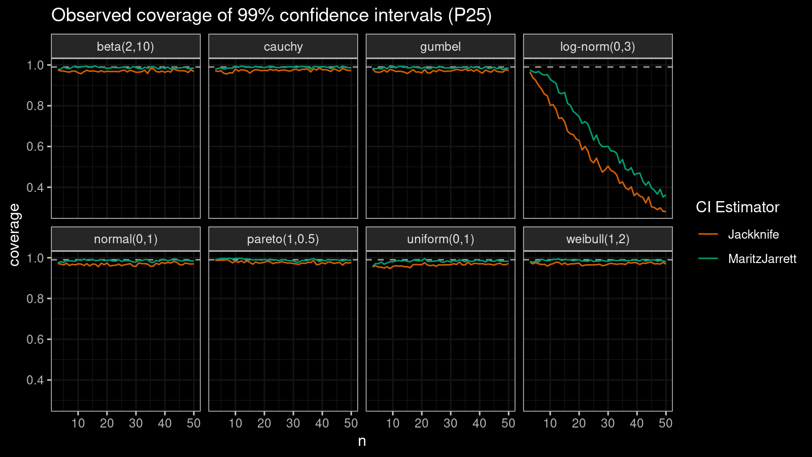
The Maritz-Jarrett method is still better.

P75

Now let’s check the $75^\textrm{th}$ percentile.

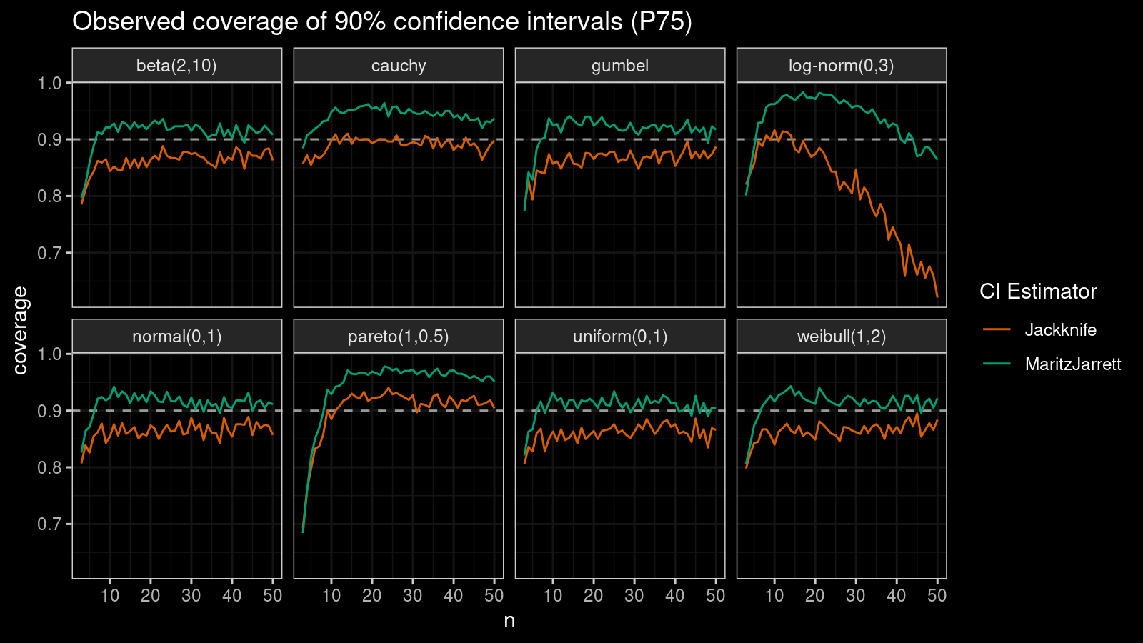
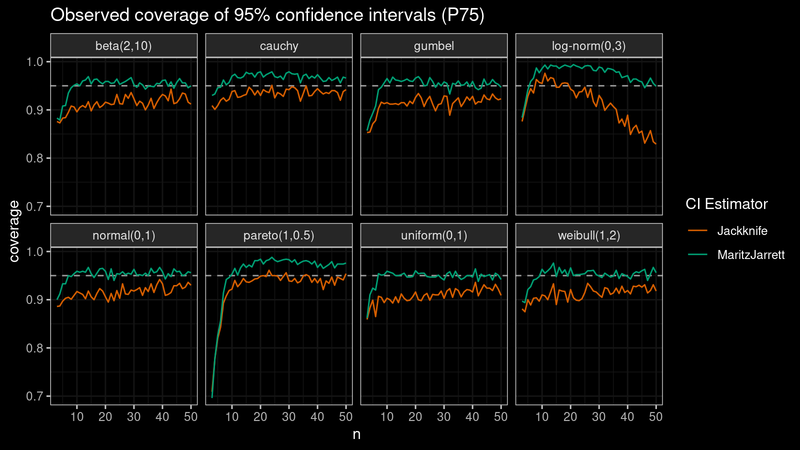
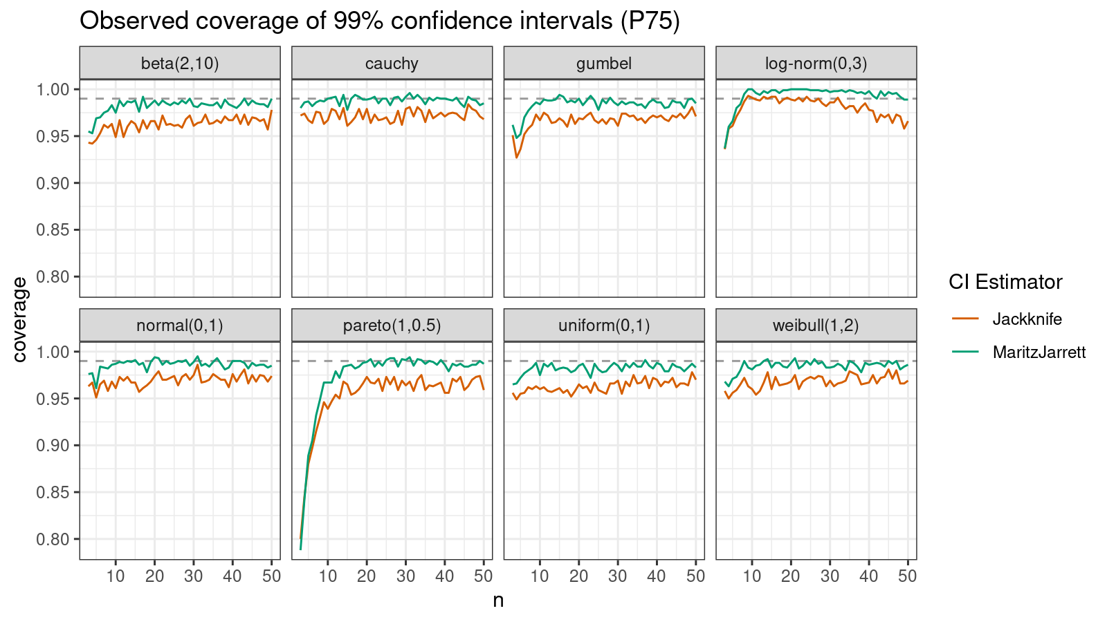
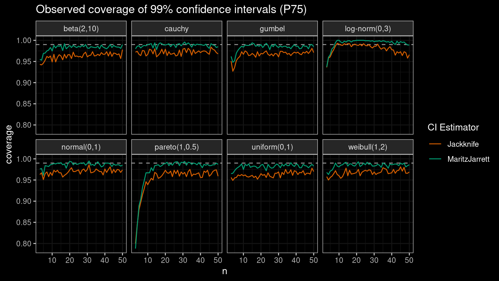
The Maritz-Jarrett method is still better.

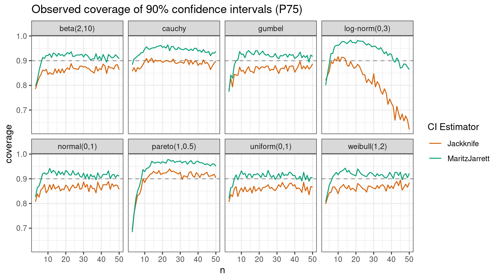
P90

Now let’s check the $90^\textrm{th}$ percentile.

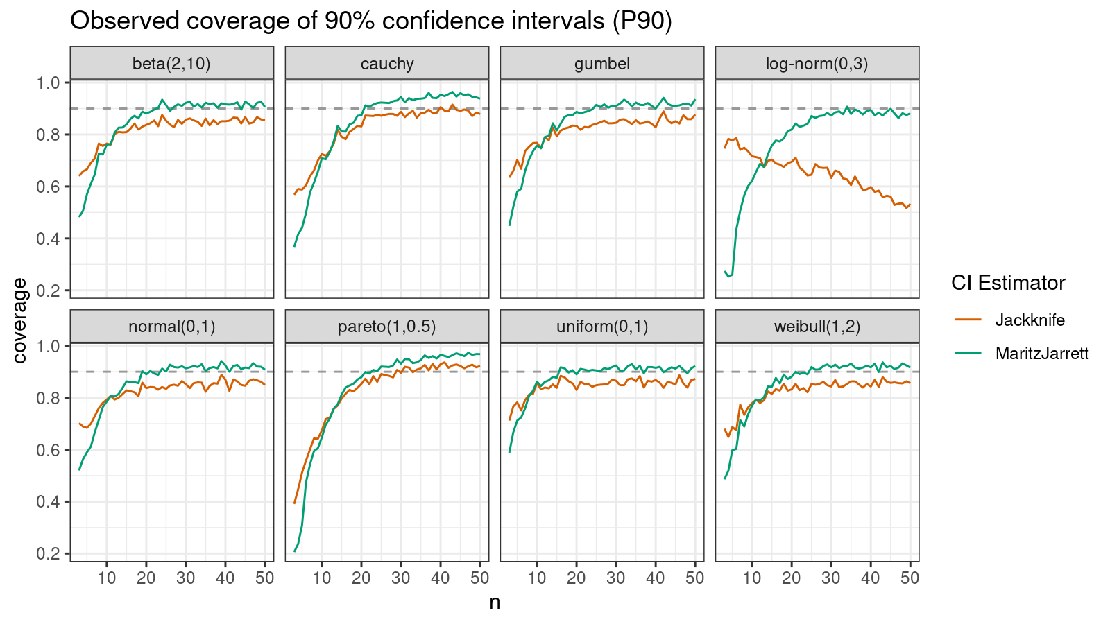
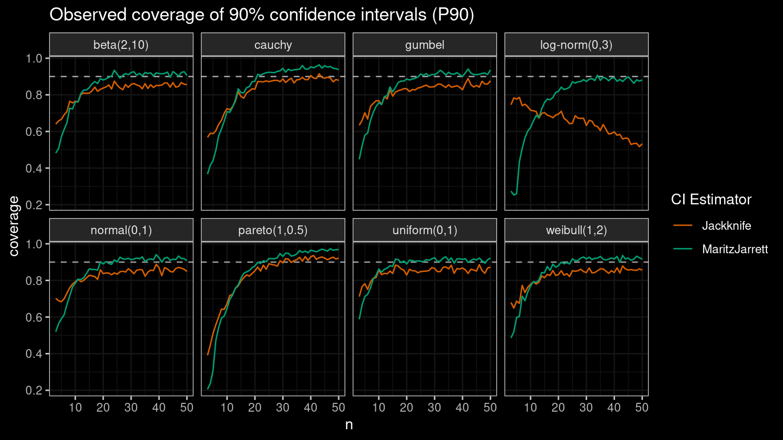
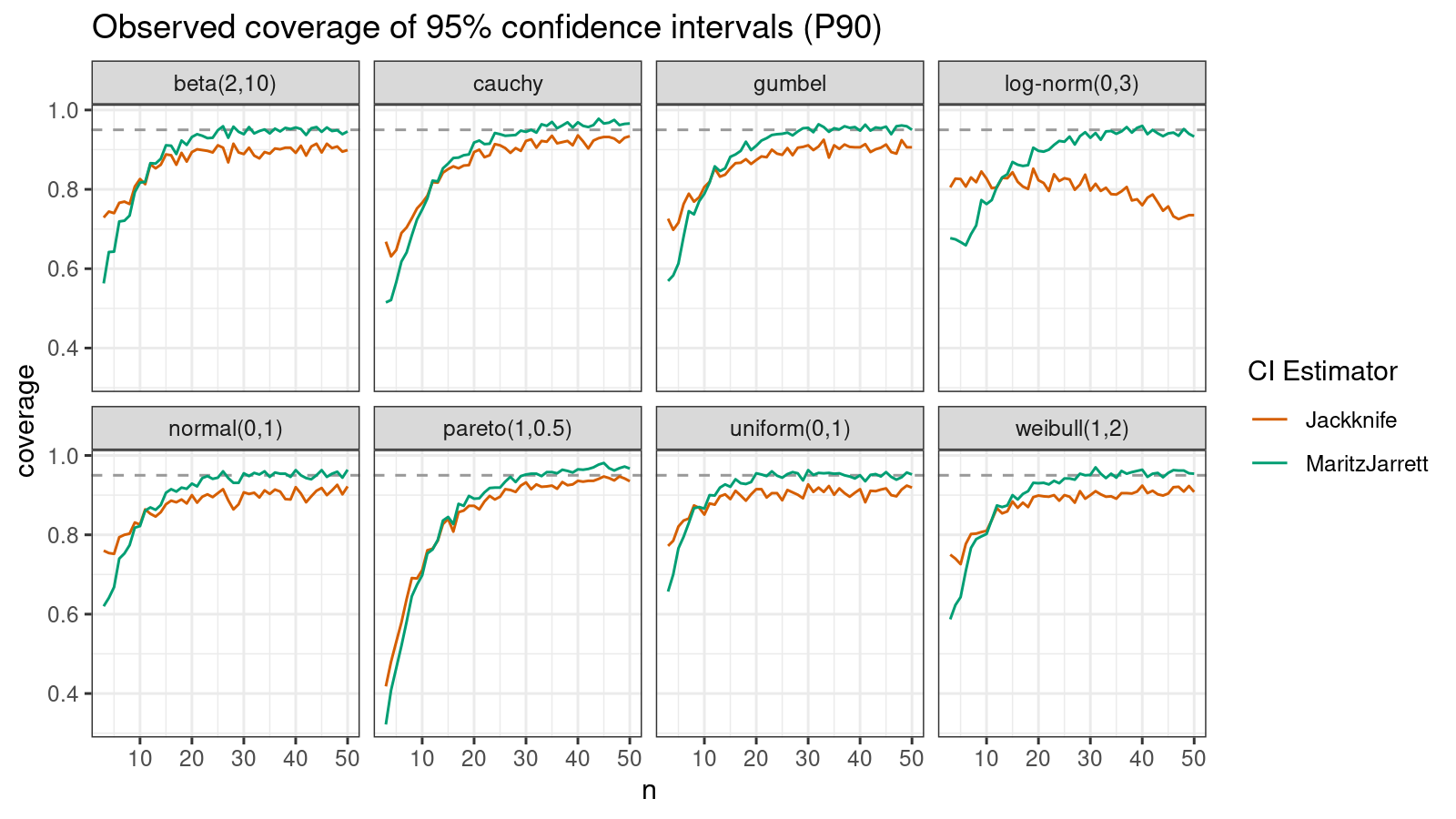
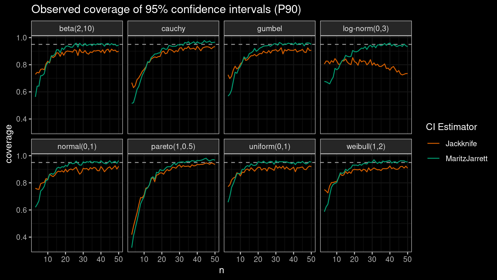
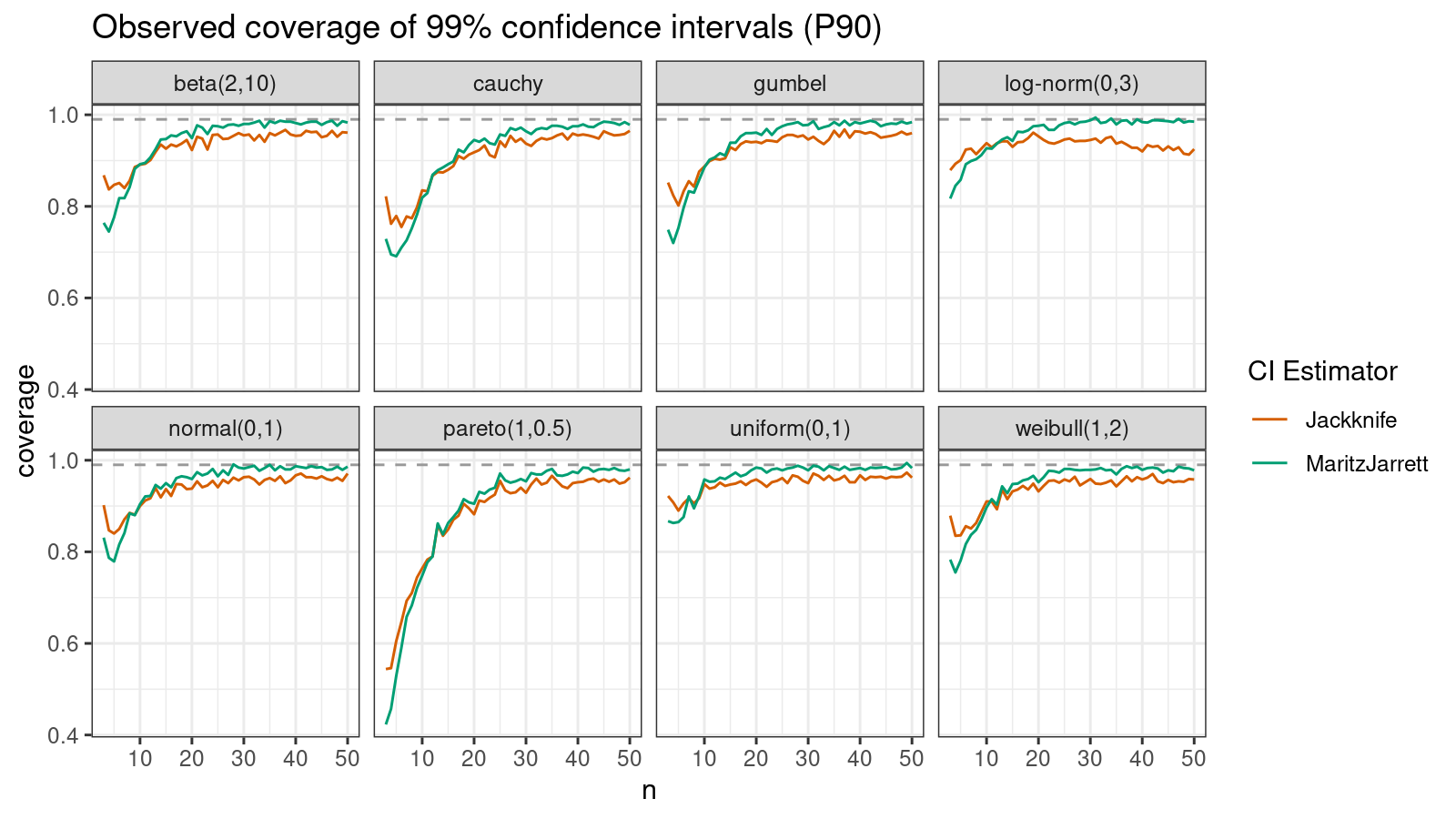
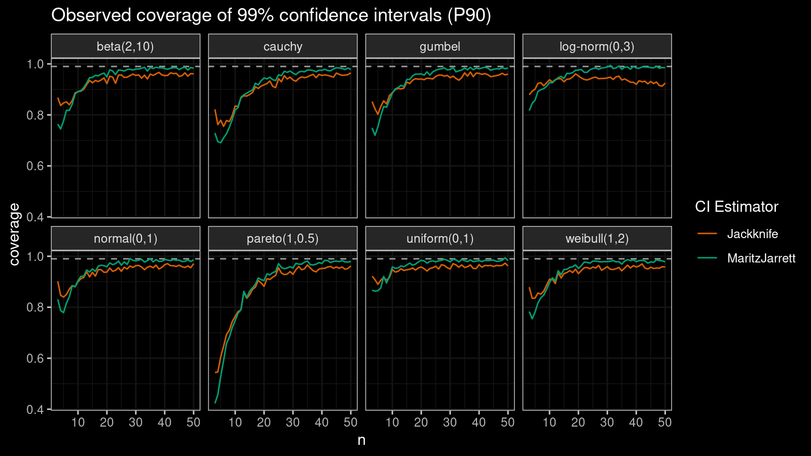
Here the situation is a little bit trickier. The jackknife method performs better for small samples ($n < 10$), but the Maritz-Jarrett method is asymptotically better.

Conclusion

In most cases, the Maritz-Jarrett method outperforms the jackknife variance estimator in terms of the confidence interval coverage. However, in some specific cases (e.g., extreme quantiles + small sample size), the jackknife approach could be more preferable.

Simulation source code

library(Hmisc)
library(evd)
library(tidyr)
library(EnvStats)

# Estimating confidence interval using the Maritz-Jarrett method
mj <- function(x, p, alpha) {
  x <- sort(x)
  n <- length(x)
  a <- p * (n + 1)
  b <- (1 - p) * (n + 1)
  cdfs <- pbeta(0:n/n, a, b)
  W <- tail(cdfs, -1) - head(cdfs, -1)
  c1 <- sum(W * x)
  c2 <- sum(W * x^2)
  se <- sqrt(c2 - c1^2)
  estimation <- c1
  margin <- se * qt(1 - (1 - alpha) / 2, df = n - 1)
  c(estimation - margin, estimation + margin)
}

# Estimating confidence interval using the jackknife approach
jk <- function(x, p, alpha) {
  n <- length(x)
  h <- hdquantile(x, p, se = T)
  estimation <- as.numeric(h)
  se <- attr(hdquantile(x, p, se = T), "se")
  margin <- se * qt(1 - (1 - alpha) / 2, df = n - 1)
  c(estimation - margin, estimation + margin)
}

check <- function(name, rfunc, qfunc, prob, alpha, iterations = 10000) {
  true.value <- qfunc(prob)
  mj.score <- 0
  jk.score <- 0
  for (i in 1:iterations) {
    x <- rfunc()
    ci.mj <- mj(x, prob, alpha)
    ci.jk <- jk(x, prob, alpha)
    if (ci.mj[1] < true.value && true.value < ci.mj[2])
      mj.score <- mj.score + 1
    if (ci.jk[1] < true.value && true.value < ci.jk[2])
      jk.score <- jk.score + 1
  }
  mj.score <- mj.score / iterations
  jk.score <- jk.score / iterations
  data.frame(
    name = name,
    n = length(rfunc()),
    "MaritzJarrett" = mj.score,
    "Jackknife" = jk.score)
}
check.single <- function(prob, alpha, n) rbind(
  check("beta(2,10)", function() rbeta(n, 2, 10), function(p) qbeta(p, 2, 10), prob, alpha),
  check("uniform(0,1)", function() runif(n), qunif, prob, alpha),
  check("normal(0,1)", function() rnorm(n), qnorm, prob, alpha),
  check("weibull(1,2)", function() rweibull(n, 2), function(p) qweibull(p, 2), prob, alpha),
  check("gumbel", function() rgumbel(n), qgumbel, prob, alpha),
  check("cauchy", function() rcauchy(n), qcauchy, prob, alpha),
  check("pareto(1,0.5)", function() rpareto(n, 1, 0.5), function(p) qpareto(p, 1, 0.5), prob, alpha),
  check("log-norm(0,3)", function() rlnorm(n, sdlog = 3), qlnorm, prob, alpha)
)
check.all <- function(prob, alpha, ns = 3:50) {
  do.call("rbind", lapply(ns, function(n) check.single(prob, alpha, n)))
}