Understanding the pitfalls of preferring the median over the mean
A common task in mathematical statistics is to aggregate a set of numbers $\mathbf{x} = \{ x_1, x_2, \ldots, x_n \}$ to a single “average” value. Such a value is usually called central tendency. There are multiple measures of central tendency. The most popular one is the arithmetic average or the mean:
$$ \overline{\mathbf{x}} = \left( x_1 + x_2 + \ldots + x_n \right) / n. $$The mean is so popular not only thanks to its simplicity but also because it provides the best way to estimate the center of the perfect normal distribution. Unfortunately, the mean is not a robust measure. This means that a single extreme value $x_i$ may distort the mean estimation and lead to a non-reproducible value that has nothing in common with the “expected” central tendency. The actual real-life distributions are never normal. They can be pretty close to the normal distribution, but only to a certain extent. Even small deviations from normality may produce occasional extreme outliers, which makes the mean an unreliable measure in the general case.
When people discover the danger of the mean, they start looking for a more robust measure of the central tendency. And the first obvious alternative is the sample median $\tilde{\mathbf{x}}$. The classic sample median is easy to calculate. First, you have to sort the sample. If the sample size $n$ is odd, the median is the middle element in the sorted sample. If $n$ is even, the median is the arithmetic average of the two middle elements in the sorted sample. The median is extremely robust: it provides a reasonable estimate even if almost half of the sample elements are corrupted.
For symmetric distributions (including the normal one), the true values of the mean and the median are the same. Once we discover the high robustness of the median, it may be tempting to always use the median instead of the mean. The median is often perceived as “something like the mean but with high resistance to outliers.” Indeed, what is the point of using the unreliable mean, if the median always provides a safer choice? Should we make the median our default option for the central tendency?
The answer is no. You should beware of any default options in mathematical statistics. All the measures are just tools, and each tool has its limitations and areas of applicability. A mindless transition from the mean to the median, regardless of the underlying distribution, is not a smart move. When we are picking a measure of central tendency to use, the first step should be reviewing the research goals: why do we need a measure of central tendency, and what are we going to do with the result? It’s impossible to make a rational decision on the statistical methods used without a clear understanding of the goals. Next, we should match the goals to the properties of available measures.
There are multiple practical issues with the median, but the most noticeable problem in practice is about its statistical efficiency. Understanding this problem reveals the price of advanced robustness of the median. In this post, we discuss the concept of statistical efficiency, estimate the statistical efficiency of the mean and the median under different distributions, and consider the Hodges-Lehmann EstimatorHodges-Lehman estimator as a measure of central tendency that provides a better trade-off between robustness and efficiency.
Sampling distribution
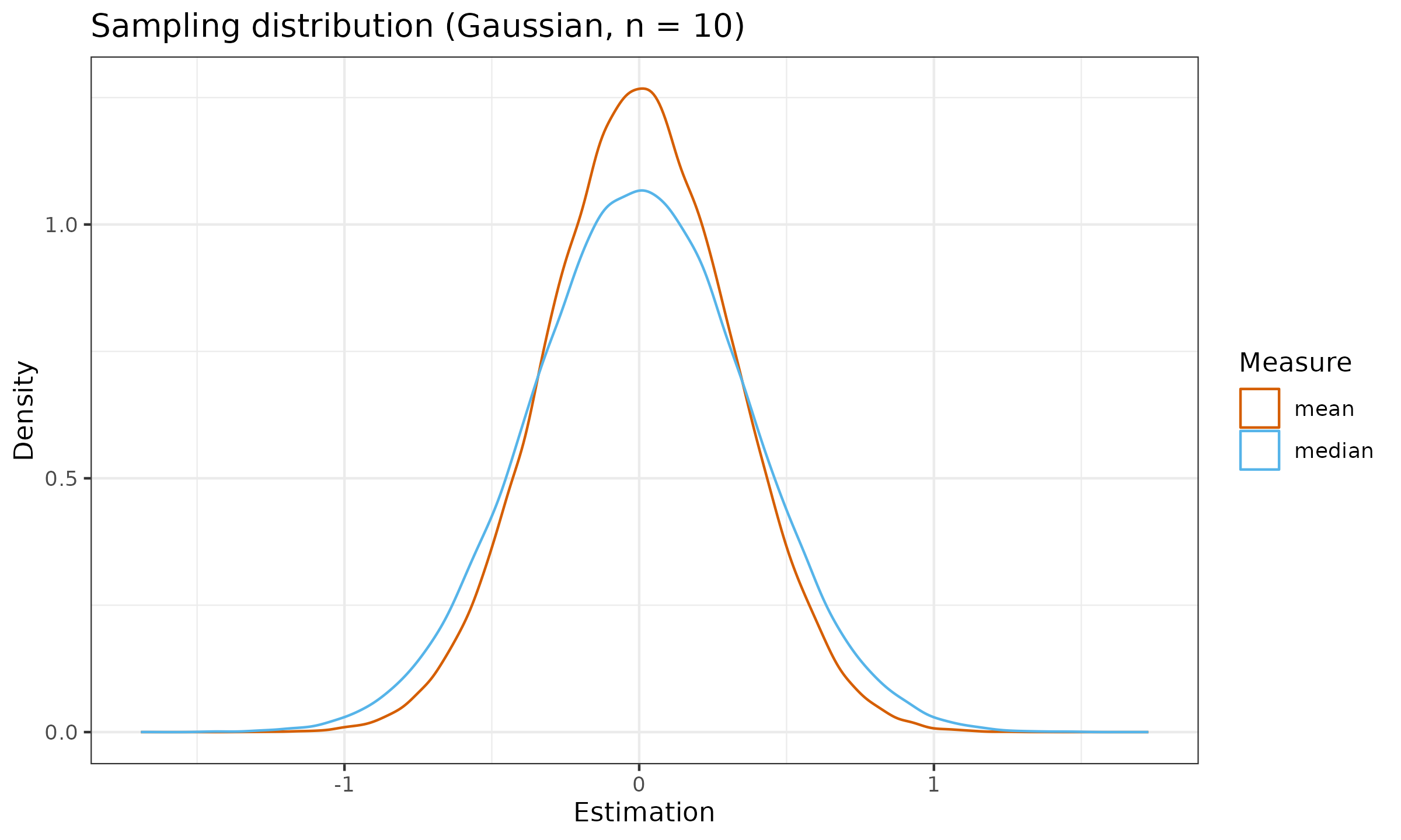
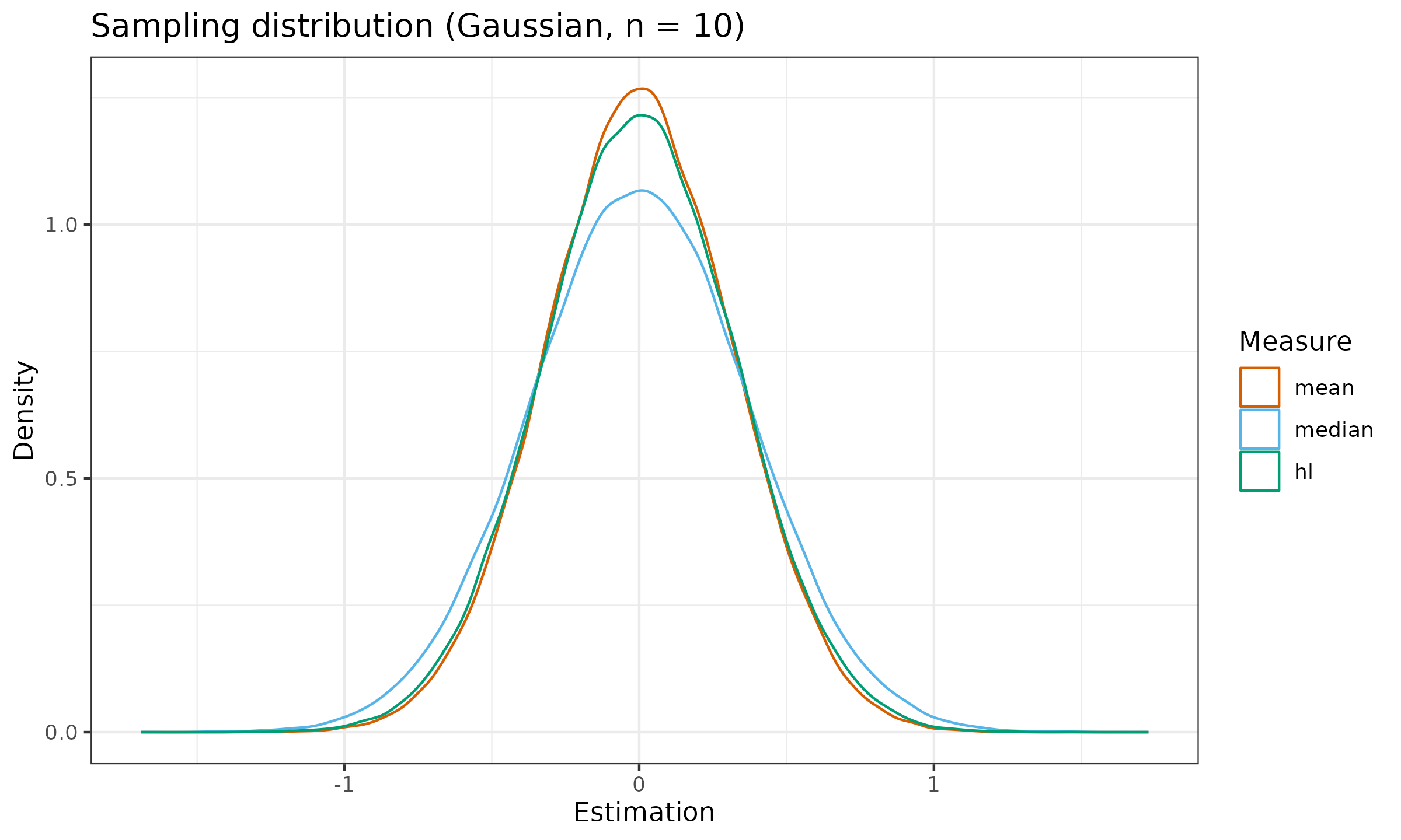
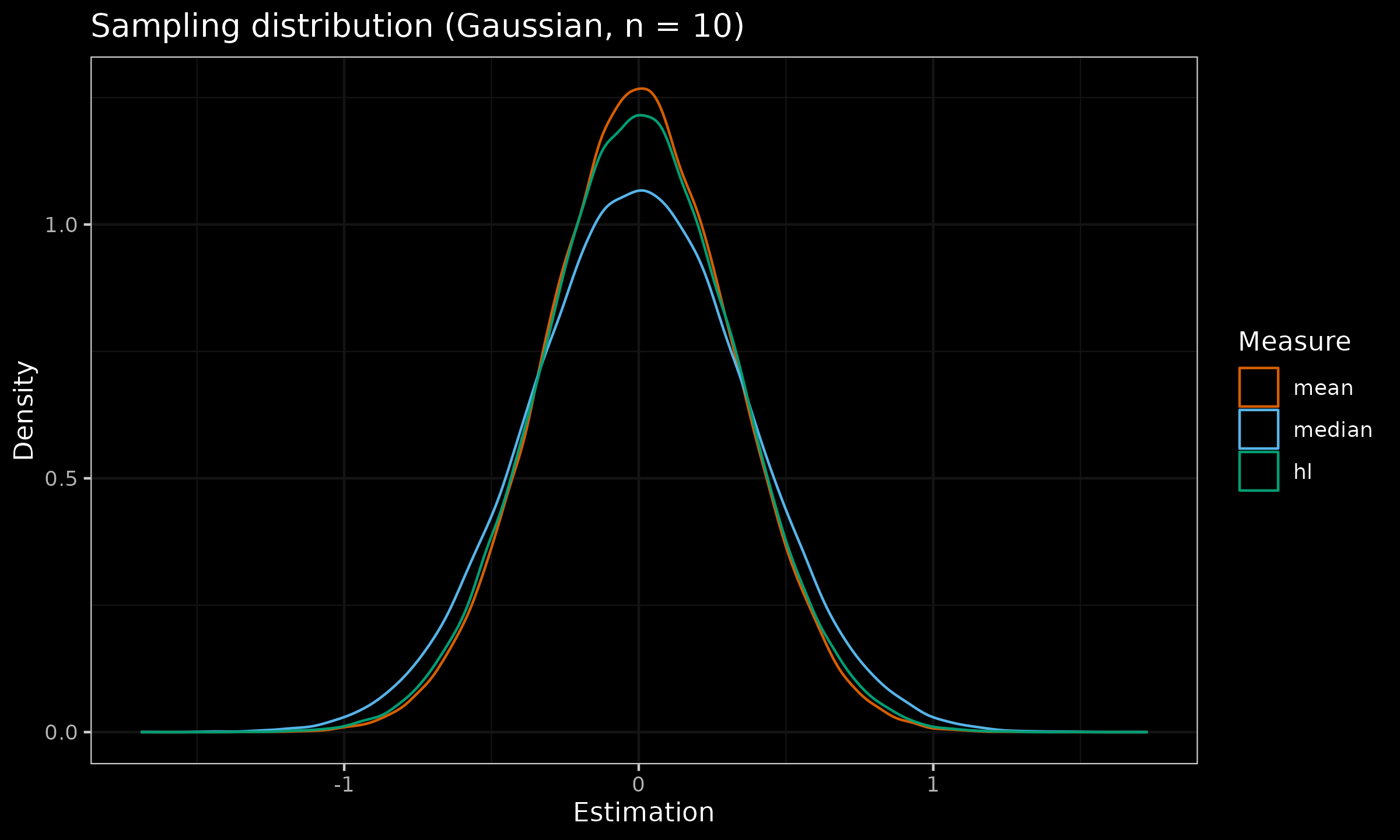
The easiest way to start exploring the properties of a measure is to build its sampling distribution. In order to do this, we should set an assumption on the actual underlying distribution of our data. For simplicity, we start with the standard normal (Gaussian) distribution $\mathcal{N}(0, 1)$. Next, we should generate multiple random samples from this underlying distribution, calculate the estimation for each sample, and build a new distribution based on these estimations.
Here are the sampling distributions of the mean and the median under the normal distribution:

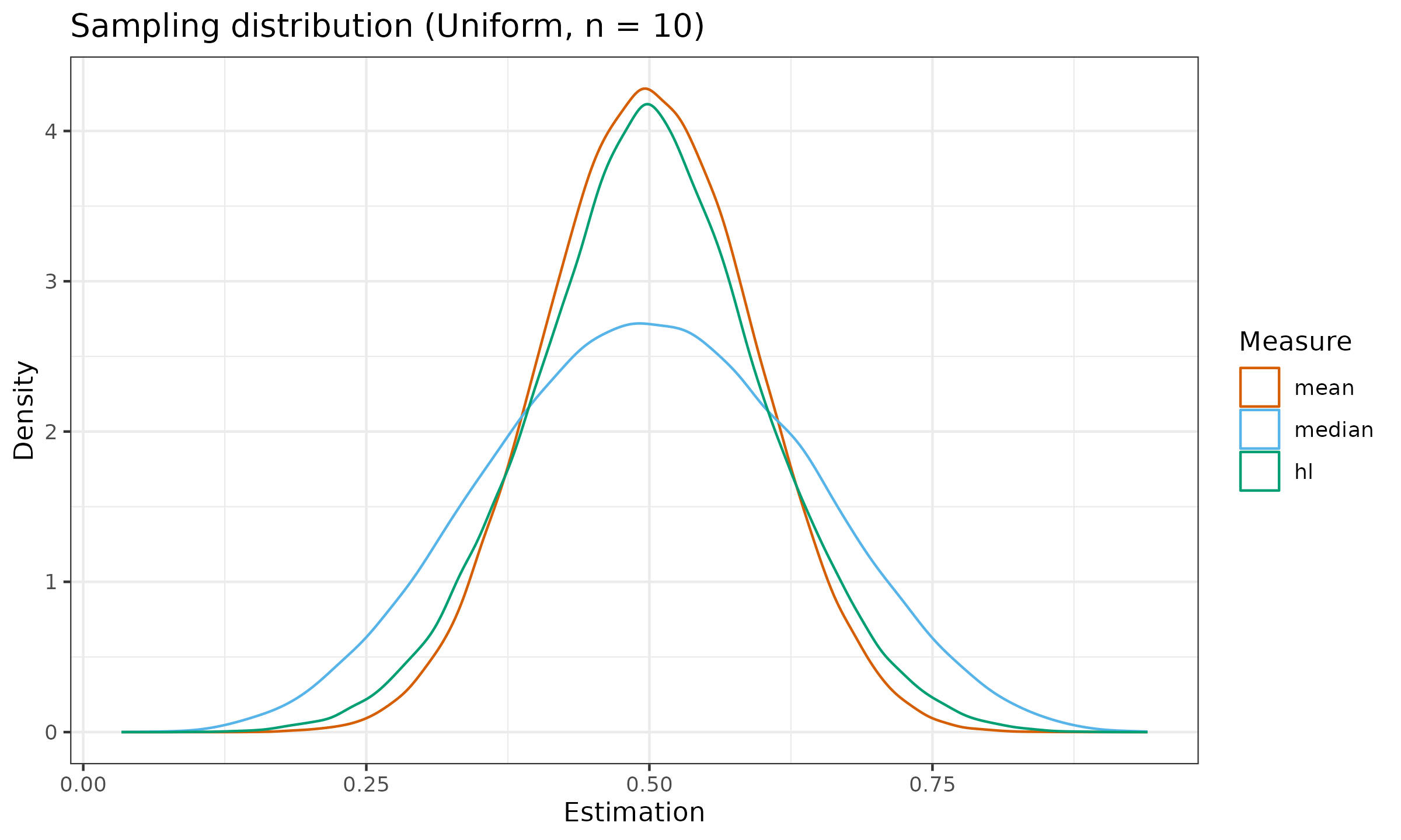
And here are the sampling distributions under the standard uniform distribution $\mathcal{U}(0, 1)$.

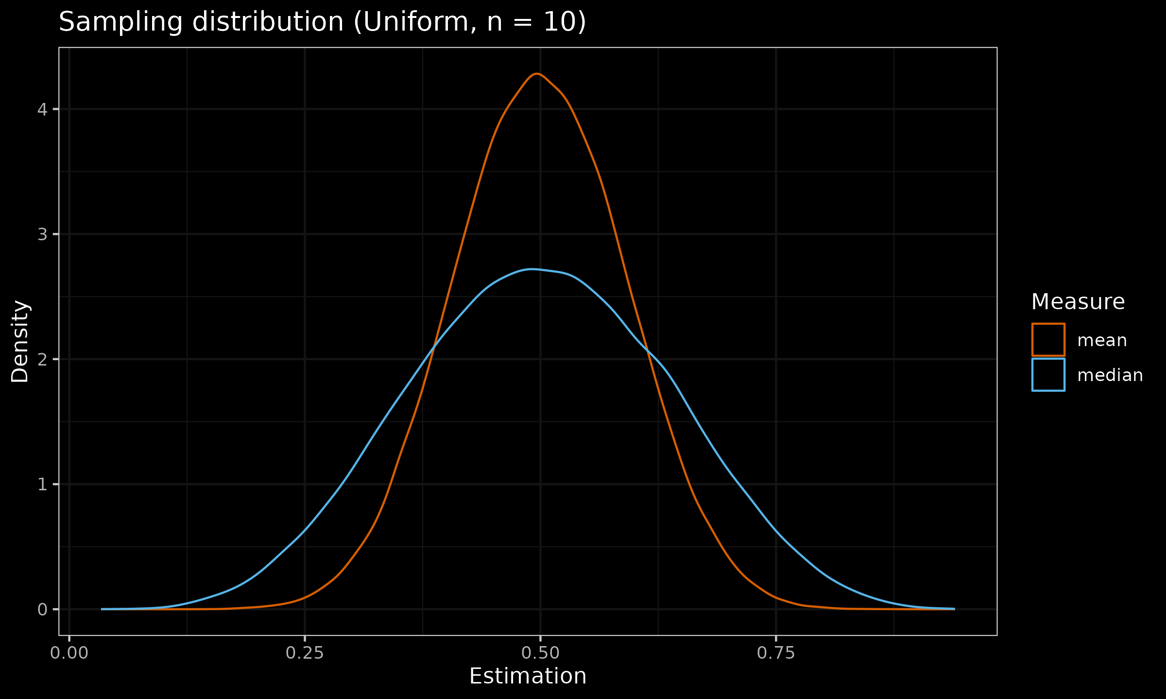
As we can see, the median sampling distribution can be noticeably wider than the mean sampling distribution (or it has larger dispersion). It is not a desired property of an estimator. The wider the sampling distribution, the less repeatable estimation we observe. In order to express the relation between sampling distribution dispersions among estimators, we have to calculate statistical efficiency.
Statistical efficiency
A common measure of statistical dispersion is the variance. The relative statistical efficiency between two estimators is defined as the ratio between variances of the corresponding sampling distributions. When the underlying distribution is the normal one, the best estimator for the central tendency is the mean: it has statistical efficiency of $100\%$. The statistical efficiency of other estimators under normality (also known as Gaussian efficiency) is typically calculated using the mean as the baseline. For an estimator $T$ (e.g., for the sample median $T=\tilde{X}$), it is defined as follows:
$$ \operatorname{eff}(T) = \frac{\mathbb{V}[\operatorname{mean}]}{\mathbb{V}[T]}, $$where $\mathbb{V}[\cdot]$ is the variance of the sampling distribution for the given estimator.
It is important to distinguish the finite-sample efficiency ($n < \infty$) and the asymptotic efficiency ($n = \infty$). While the case of $n = \infty$ is practically impossible, the asymptotic efficiency provides an acceptable efficiency approximation for large samples. However, when we consider small samples, it is important to consider the finite-sample efficiency separately since it can noticeably differ from its asymptotic limit.
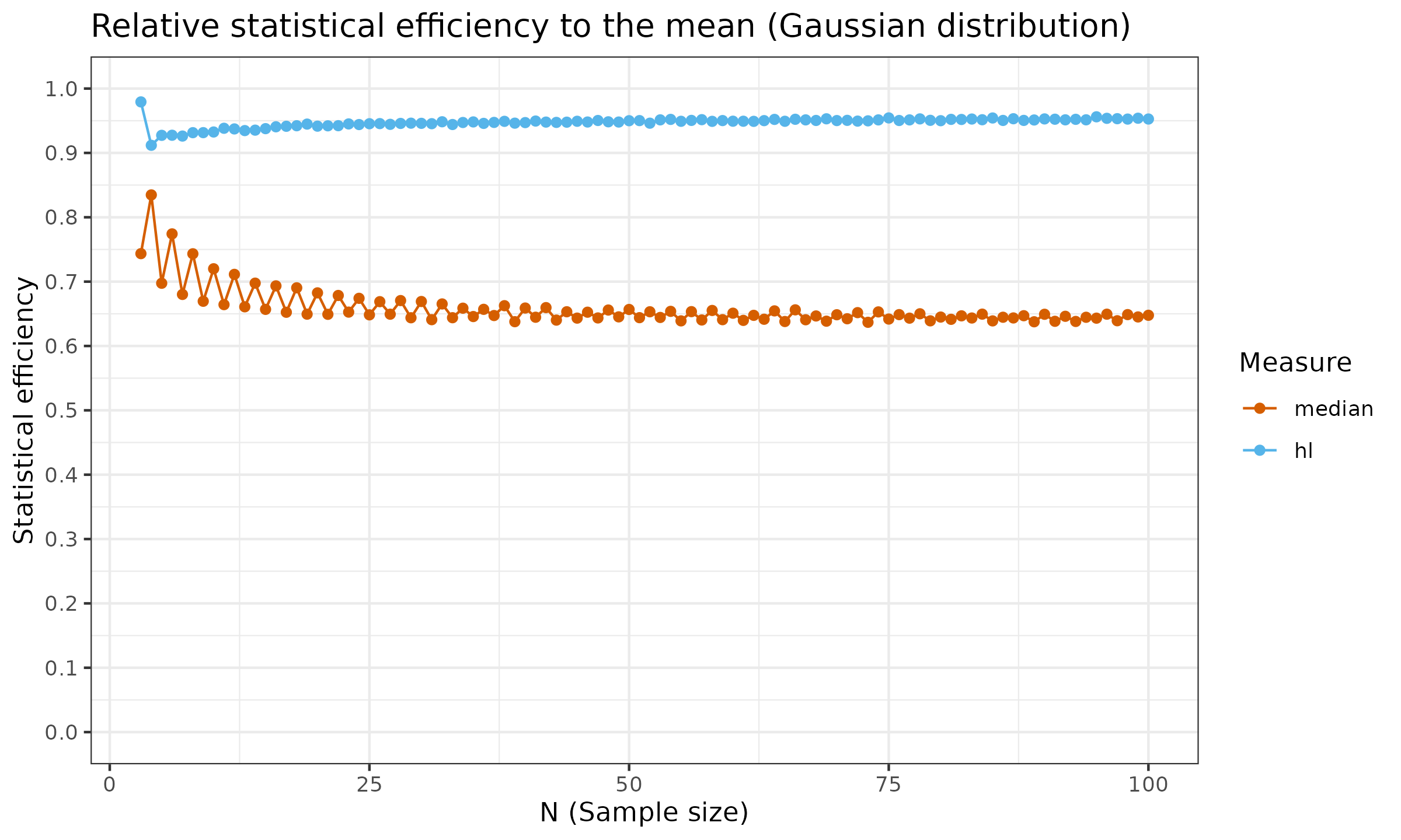
For the sample median, the asymptotic Gaussian efficiency is $\approx 64\%$. The sample median relative efficiency to the mean under the uniform distribution is $\approx 34\%$. The finite-sample efficiency values are presented in the below charts (the presented estimation are not precise and has some noise, but the common trend is clear):

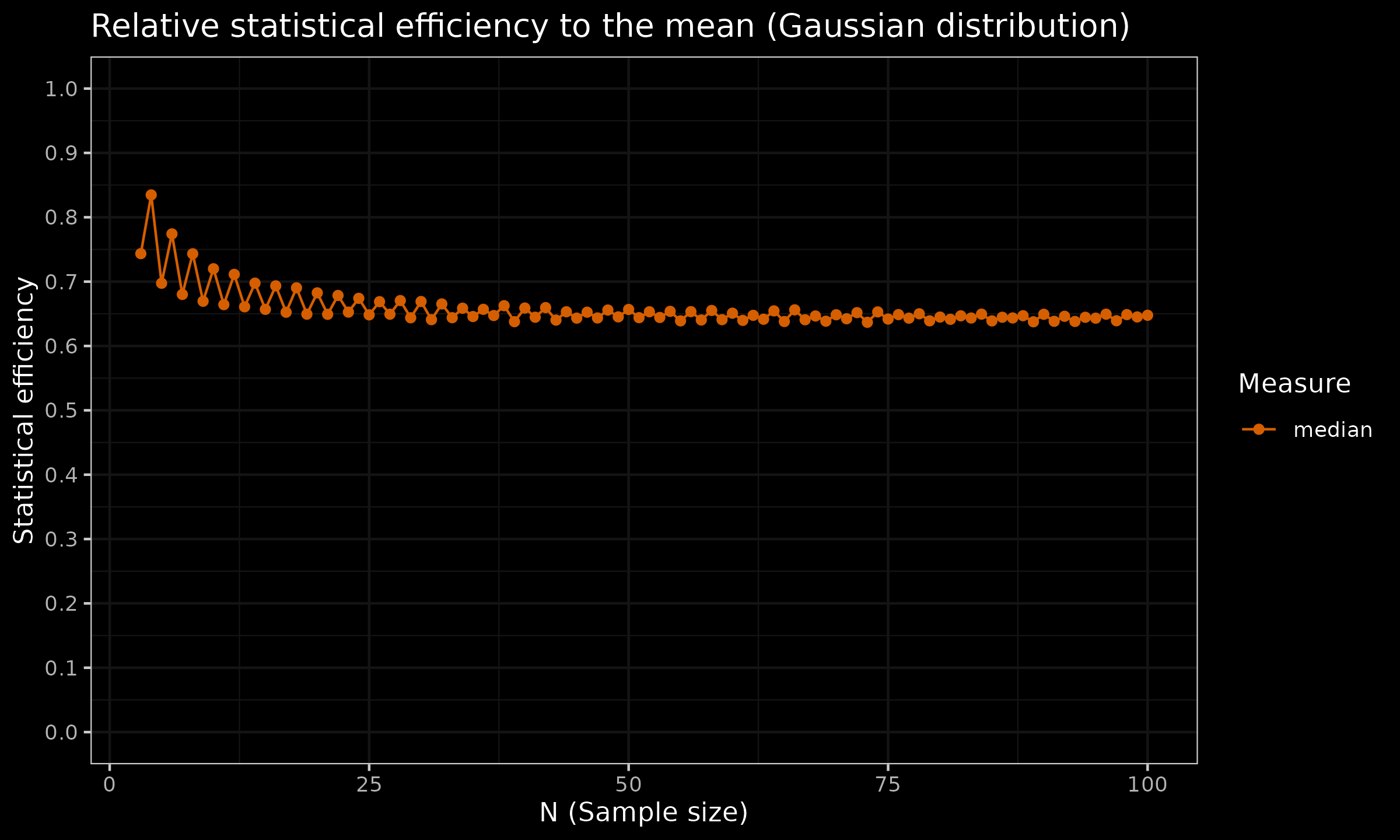
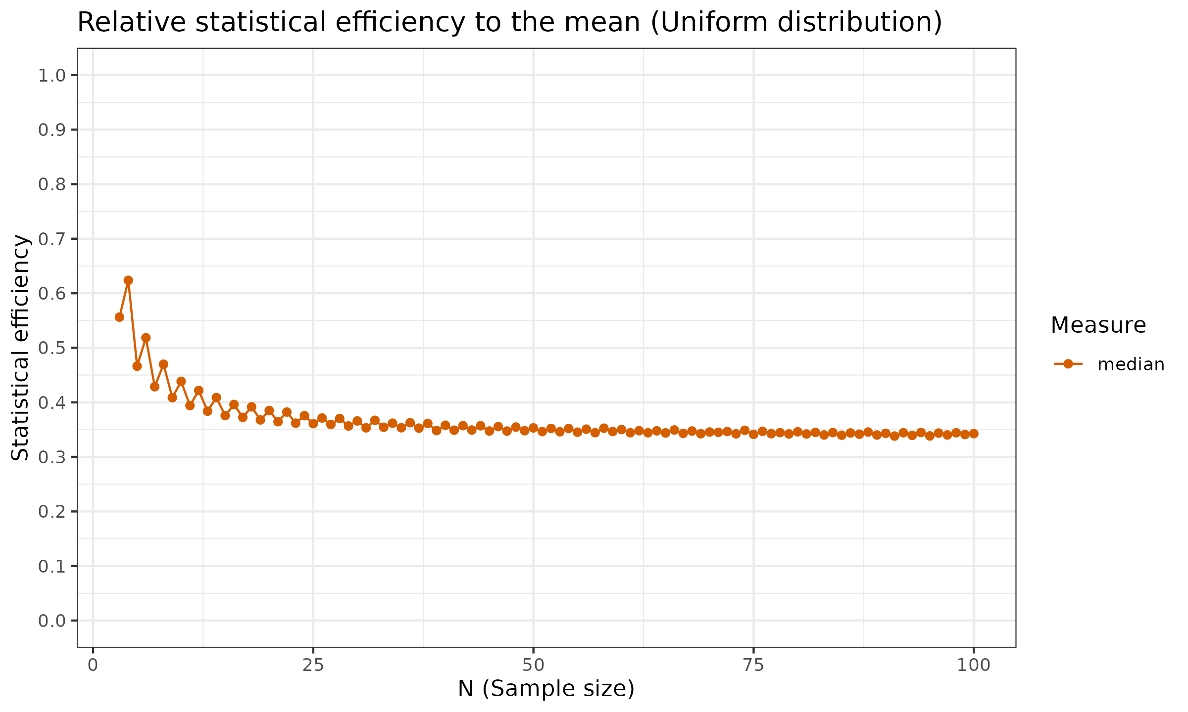

As we can see, the robustness of the median doesn’t come for free: it has a price in the form of reduced statistical efficiency. Therefore, if the underlying distribution is light-tailed and no huge outliers are expected, switching to the sample median as a measure of central tendency is not always a good move.
It is worth noting that there are other measures of central tendency with other properties. Let us say that we expect some outliers, but not so many of them (definitely, much less than $50\%$ of the sample). We cannot use the mean since it can be corrupted by these outliers. However, we don’t want to use the sample median either since we will get a huge efficiency loss. What should we do? One of the possible solutions is the Hodges-Lehmann location estimator.
Hodges-Lehmann location estimator
The Hodges-Lehmann location estimator (also known as pseudo-median) is a robust, non-parametric statistic used as a measure of the central tendency. For a sample $\mathbf{x} = \{ x_1, x_2, \ldots, x_n \}$, it is defined as the median of the Walsh (pairwise) averages:
$$ \operatorname{HL}(\mathbf{x}) = \underset{1 \leq i \leq j \leq n}{\operatorname{median}} \left(\frac{x_i + x_j}{2} \right). $$Now let us compare the sampling distribution and the statistical efficiency of the Hodges-Lehmann location estimator against the median and the mean:

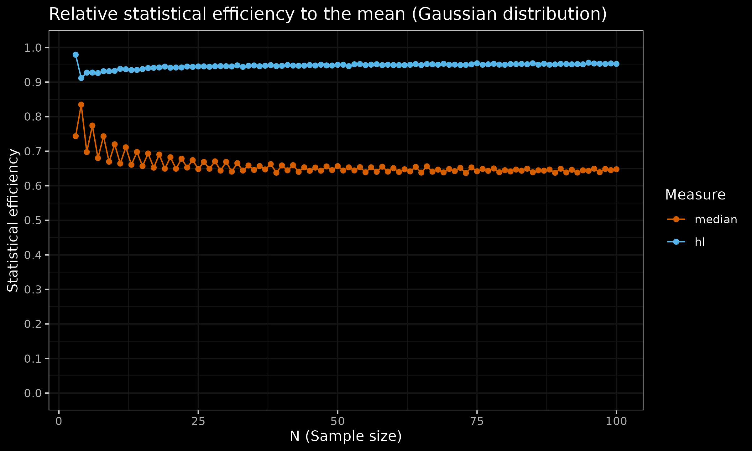
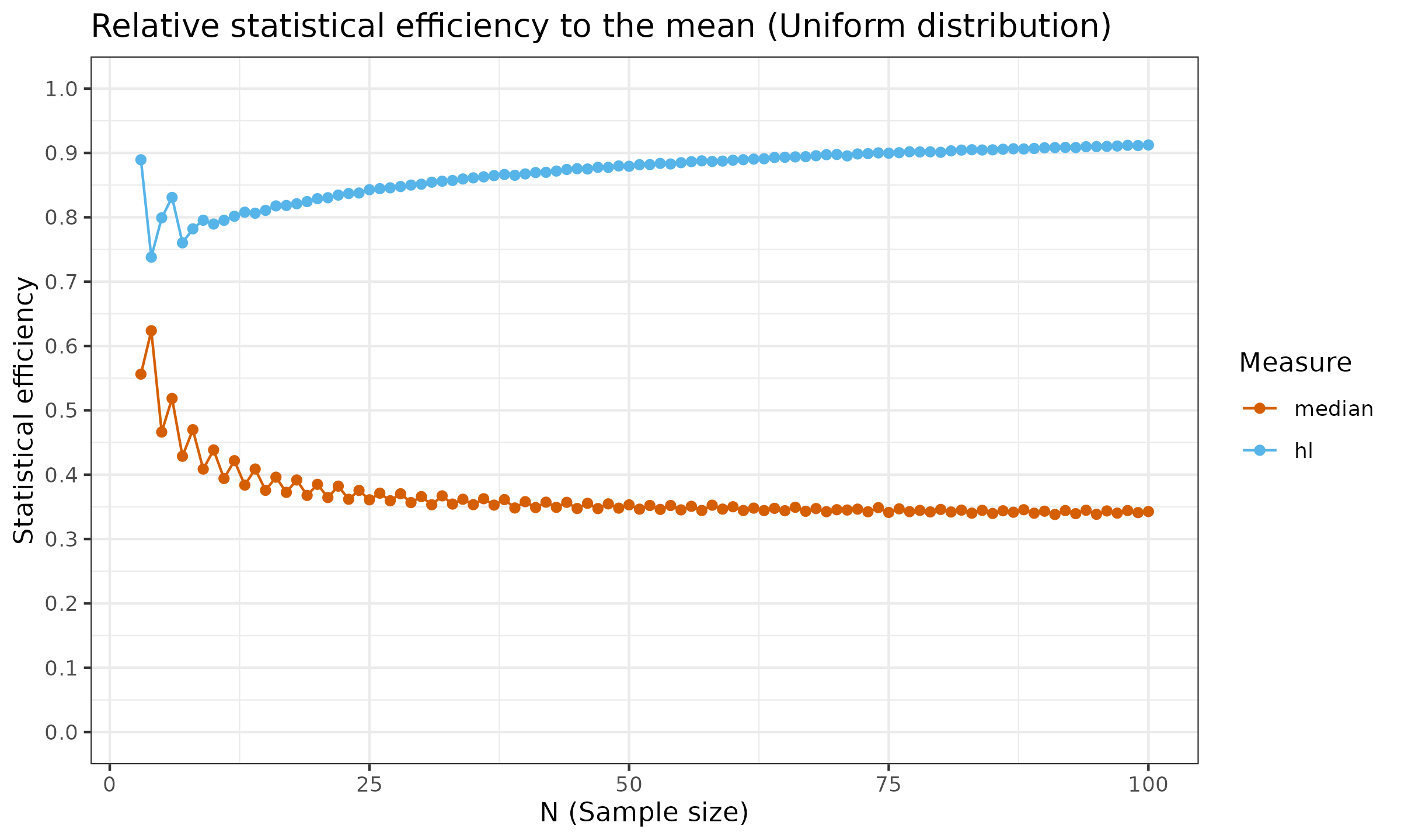
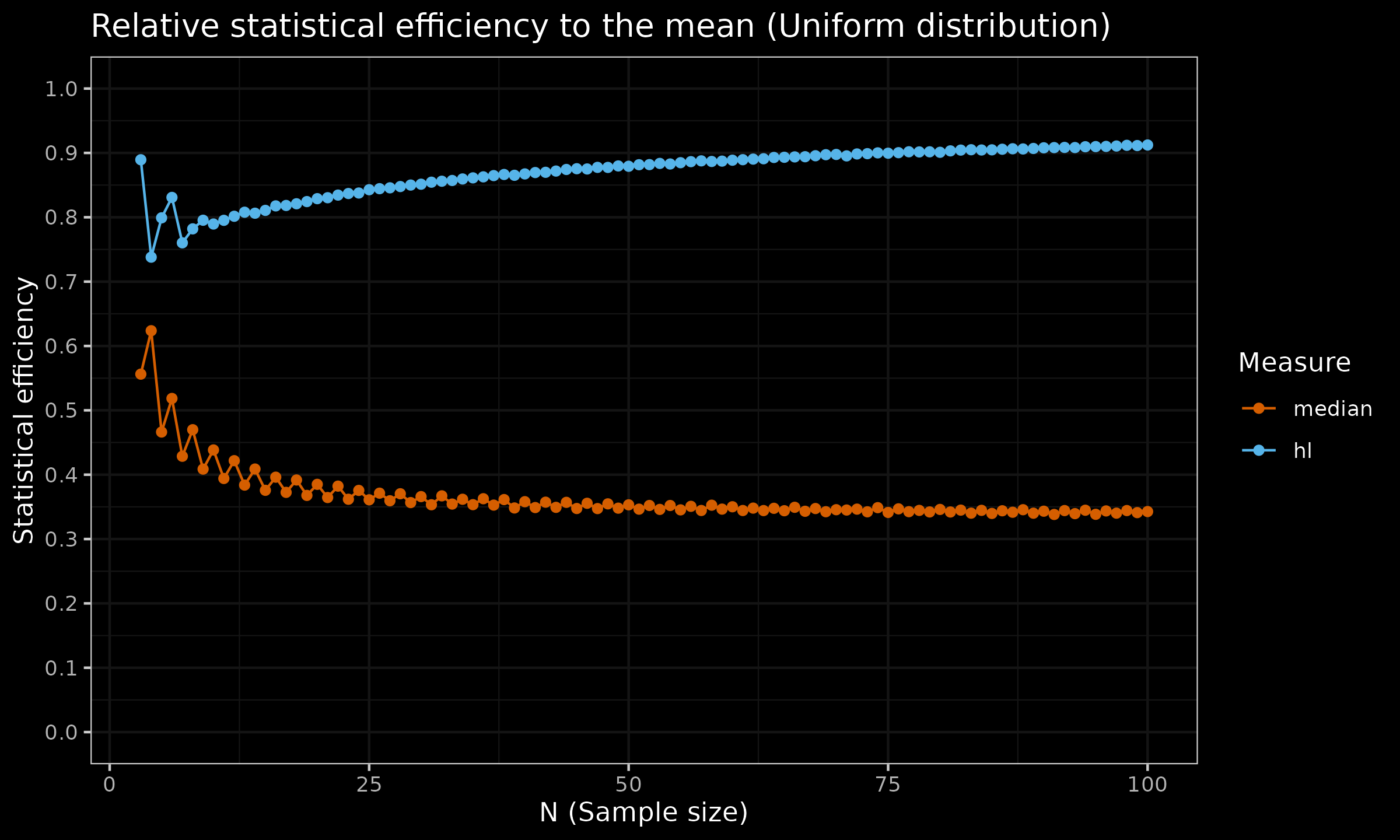
As we can see, the Hodges-Lehmann is much closer to the mean than the median. To be more specific, the asymptotic Gaussian efficiency of $\operatorname{HL}$ is $\approx 96\%$, which is much better than $\approx 64\%$ for the sample median. For the uniform distribution, the Gaussian efficiency of $\operatorname{HL}$ is also close to $1.0$, while the sample median has an efficiency of $\approx 34\%$.
Meanwhile, the Hodges-Lehmann location estimator has decent robustness: its asymptotic breakdown point is $\approx 29\%$. This means that even $\approx 29\%$ of the sample is corrupted by outliers, $\operatorname{HL}$ will still provide a reasonable estimate. This makes $\operatorname{HL}$ a decent alternative to the sample median.
Conclusion
In summary, choosing a measure of central tendency in mathematical statistics requires careful analysis of the dataset and the research goals. While the mean is simple and efficient, it’s sensitive to outliers. On the other hand, the median is robust but lacks statistical efficiency. Thus, neither should be a default choice. Instead, depending on the situation, using other options like the Hodges-Lehmann location estimator could be better because it balances robustness and efficiency.