Misleading geometric mean

There are multiple ways to compute the “average” value of an array of numbers. One of such ways is the geometric mean. For a sample $x = \{ x_1, x_2, \ldots, x_n \}$, the geometric means is defined as follows:

This approach is widely recommended for some specific tasks. Let’s say we want to compare the performance of two machines $M_x$ and $M_y$. In order to do this, we design a set of benchmarks $b = \{b_1, b_2, \ldots, b_n \}$ and obtain two sets of measurements $x = \{ x_1, x_2, \ldots, x_n \}$ and $y = \{ y_1, y_2, \ldots, y_n \}$. Once we have these two samples, we may have a desire to express the difference between two machines as a single number and get a conclusion like “Machine $M_y$ works two times faster than $M_x$.” I think that this approach is flawed because such a difference couldn’t be expressed as a single number: the result heavily depends on the workloads that we analyze. For example, imagine that $M_x$ is a machine with HDD and fast CPU, $M_y$ is a machine with SSD and slow CPU. In this case, $M_x$ could be faster on CPU-bound workloads while $M_y$ could be faster on disk-bound workloads. I really like this summary from “Notes on Calculating Computer Performance” by Bruce Jacob and Trevor Mudge (in the same paper, the authors criticize the approach with the geometric mean):

Performance is therefore not a single number, but really a collection of implications. It is nothing more or less than the measure of how much time we save running our tests on the machines in question. If someone else has similar needs to ours, our performance numbers will be useful to them. However, two people with different sets of criteria will likely walk away with two completely different performance numbers for the same machine.

However, some other authors (e.g., “How not to lie with statistics: the correct way to summarize benchmark results”) actually recommend using the geometric mean to get such a number that describes the performance ratio of $M_x$ and $M_y$. I have to admit that the geometric mean could provide a reasonable result in some simple cases. Indeed, on normalized numbers, it works much better than the arithmetic mean (that provides meaningless result) because of its nice property: $\operatorname{GM}(x_i/y_i) = \operatorname{GM}(x_i) / \operatorname{GM}(y_i)$. However, it doesn’t work properly in the general case. Firstly, the desire to express the difference between two machines is vicious: the result heavily depends on the chosen workloads. Secondly, the performance of a single benchmark $b_i$ couldn’t be described as a single number $x_i$: we should consider the whole performance distributions. In order to describe the difference between two distributions, we could consider the shift and ration functions (that work much better than the shift and ratio distributions).

Even if you consider a pretty homogenous set of benchmarks and all the distributions are pretty narrow, the geometric mean has severe drawbacks that you should keep in mind. In this post, I briefly cover some of these drawbacks and highlight problems that you may have if you use this metric.

Computational problems

If $n$ is large, the straightforward way to compute the geometric mean may lead to a low accuracy due to overflow in the product $x_1 x_2 \ldots x_n$. This problem is a non-critical one because it could be easily solved using the exponential form of the geometric mean:

Zero values

The usage of geometric mean makes sense only for positive numbers. However, in real life, we may get a situation when our samples contain zero values. If we discuss $\operatorname{GM}$ in the context of software benchmarks, we may have zero because of poor benchmark design (if we forget to use the benchmark result, the compiler may eliminate the benchmark body) or small granularity of our measurements (e.g., we express the measurements in milliseconds, but a benchmark takes less than 1 millisecond). It’s enough to get a single zero measurement to completely spoil the final results. If $x_1=0$, $\operatorname{GM}(x)=0$ regardless of other $x_i$ values.

Non-stability on small values

We shouldn’t consider the ratio of the geometric means as a stable indicator of the true ratio (especially when the sample elements are small).

Let’s say that we randomly take two samples of size $100$ from the standard uniform distribution $\mathcal{U}(0,1)$ and calculate the ratio of the corresponding geometric means $\operatorname{GM}(x_i) / \operatorname{GM}(y_i)$. Using the below R snippet, I have performed this experiment $1000$ times:

gm <- function(x) exp(mean(log(x)))
set.seed(42)
u <- sort(replicate(1000, gm(runif(100)) / gm(runif(100))))

Here are the TOP 5 lowest and the TOP 5 highest results:

> head(u, 5)
[1] 0.6367051 0.6471006 0.6783169 0.6809434 0.6845263
> tail(u, 5)
[1] 1.464806 1.468903 1.495844 1.519174 1.520818

As we can see, the obtained ratio goes from $\approx 0.6$ to $\approx 1.5$ while both samples had been taken from the same distribution and the sample size is quite large ($n=100$). Thus, we shouldn’t always interpret $\operatorname{GM}(x_i) / \operatorname{GM}(y_i) = 1.5$ as 1.5x difference between distributions $X$ and $Y$: such a value could be easily observed by chance without the actual difference between $X$ and $Y$.

Robustness

While the geometric mean is much more resistant to outliers than the arithmetic mean, it’s not robust. It means that a single outlier could corrupt our result.

Let’s consider the Weibull distribution with $\textrm{shape}=0.1$ (which is a heavy-tailed distribution):

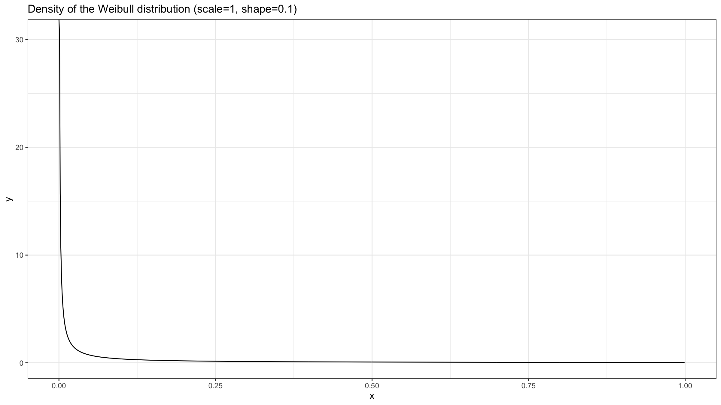
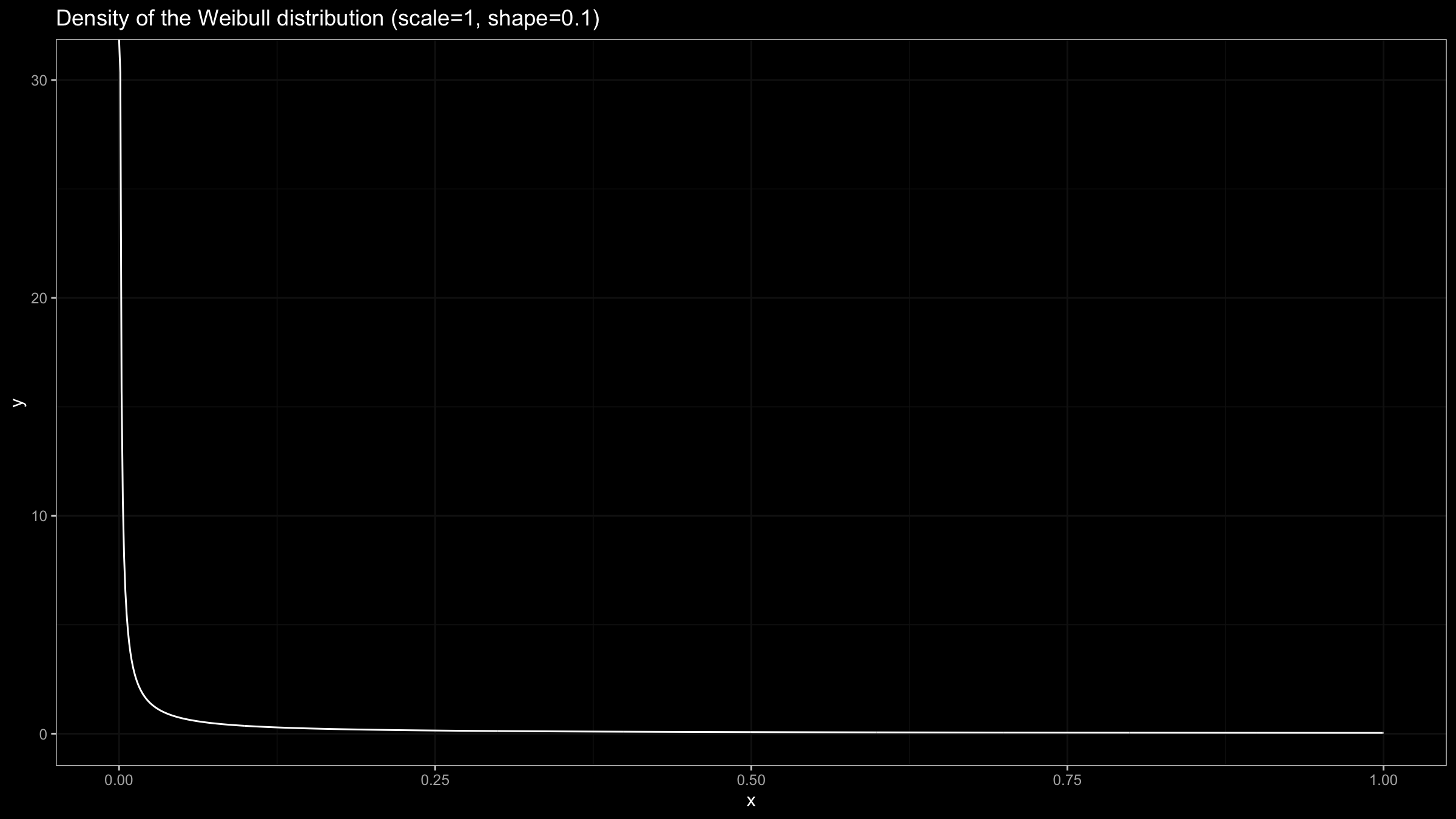
Next, let’s perform the experiment from the previous section using the Weibull distribution:

library(evd)
set.seed(42)
u <- sort(replicate(1000, gm(rweibull(100, 0.1)) / gm(rweibull(100, 0.1))))

Here are the TOP 5 lowest and the TOP 5 highest results:

> head(u, 5)
[1] 0.001484348 0.004923385 0.005668490 0.006009496 0.006248911
> tail(u, 5)
[1] 131.4244 200.4754 242.1431 273.2267 312.9481

While both samples had been taken from the same distribution, the corresponding geometric mean ratio could be $\approx 0.001$ or $\approx 300$ which is pretty far from the expected $1$.

Performance distributions are often heavy-tailed, the corresponding samples may contain extreme outliers. We should remember that such outliers could completely distort our conclusions if they are not handled properly.

Conclusion

We shouldn’t consider the geometric mean as a universal approach to compare two sets of numbers. While it may work fine in some applications, it doesn’t produce reliable results in the general case. I recommend avoiding aggregation values to a single number and considering the whole distributions.