Misleading kurtosis

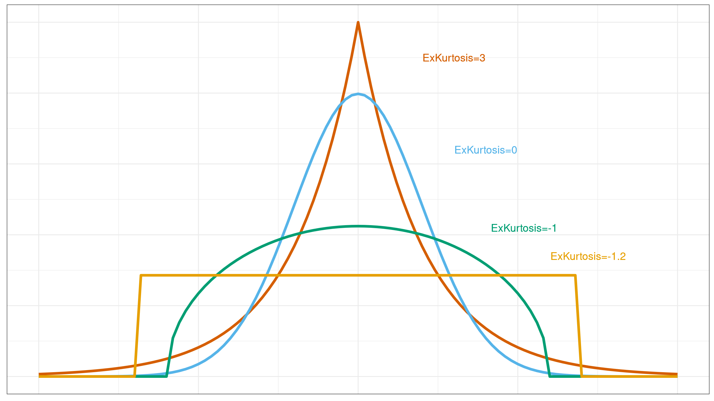
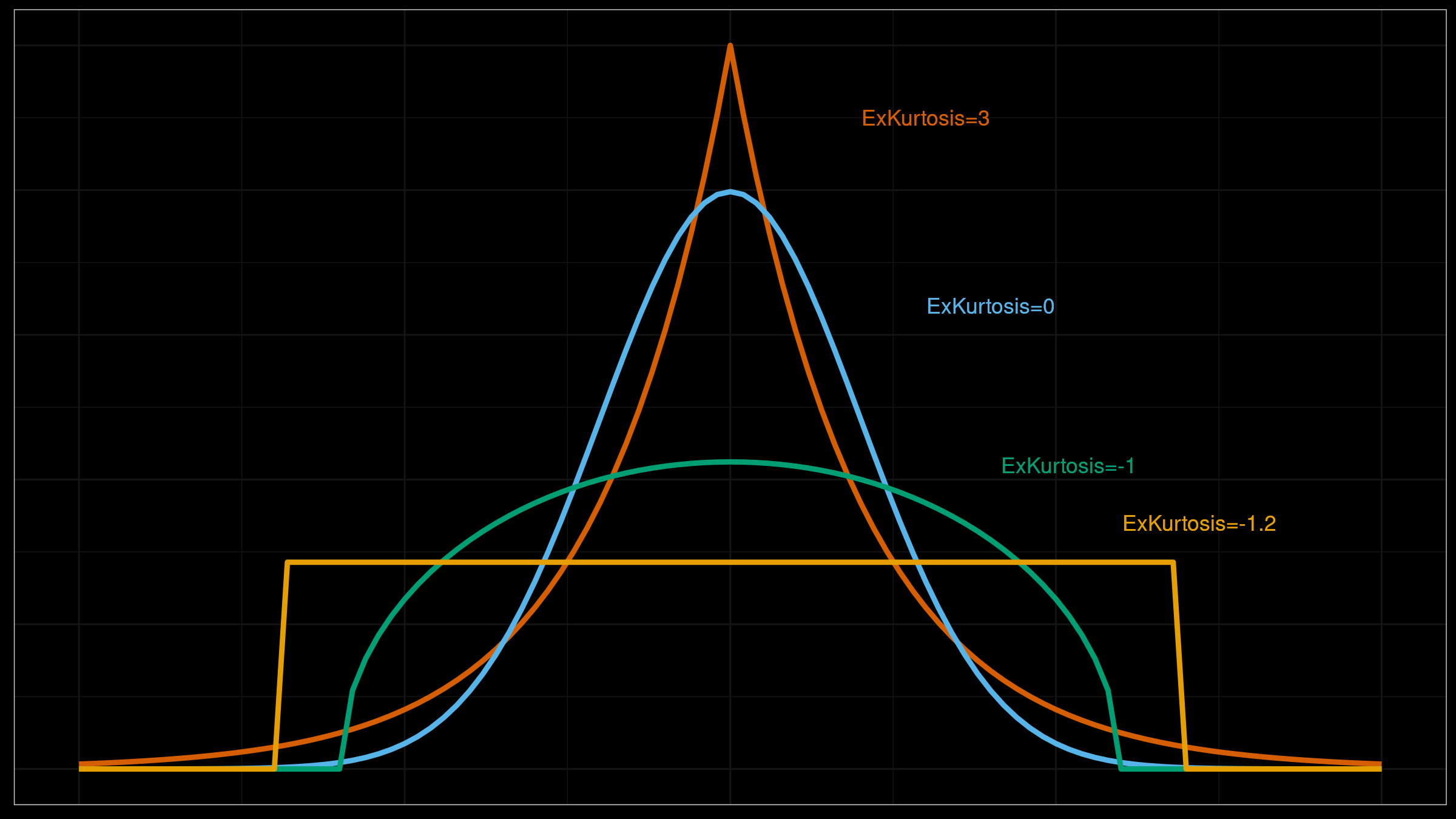
I already discussed misleadingness of such metrics like standard deviation and skewness. It’s time to discuss misleadingness of the measure of tailedness: kurtosis (which, sometimes, could be incorrectly interpreted as a measure of peakedness). Typically, the concept of kurtosis is explained with the help of images like this:

Unfortunately, the raw kurtosis value may provide wrong insights about distribution properties. In this post, we briefly discuss the sources of its misleadingness:

• There are multiple definitions of kurtosis. The most significant confusion arises between “kurtosis” and “excess kurtosis,” but there are other definitions of this measure.
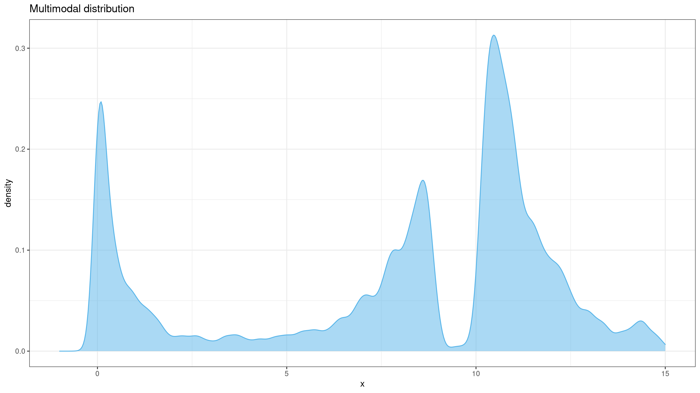
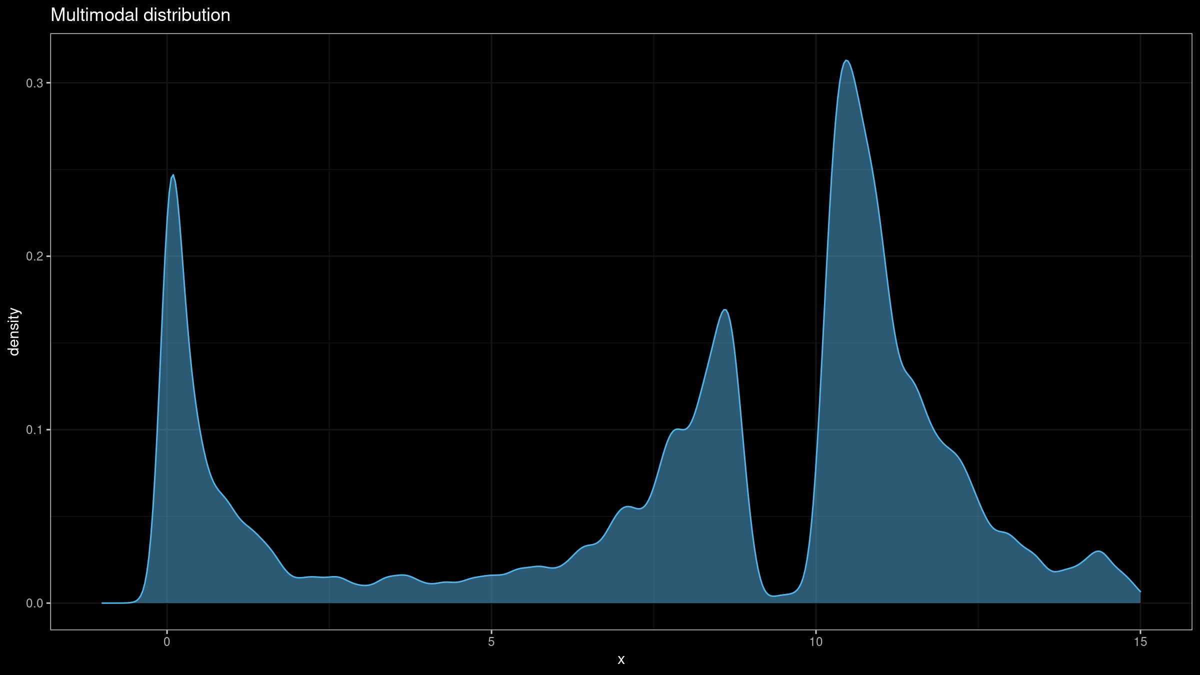
• Kurtosis may work fine for unimodal distributions, but it performs not so clear for multimodal distributions.
• The classic definition of kurtosis is not robust: it could be easily spoiled by extreme outliers.

Multiple Definitions

The classic kurtosis of a distribution $X$ is typically defined as the fourth standardized moment:

For the standard normal distribution, $\operatorname{Kurt}(\mathcal{N}(0, 1)) = 3$. This “default” value is not convenient. Thus, many people use so-called “excess kurtosis” instead of the original one:

For the standard normal distribution, $\operatorname{Kurt}'(\mathcal{N}(0, 1)) = 0$, which makes it a more handy way to work with the metric. Unfortunately, people often omit the “excess” word and refer $\operatorname{Kurt}$ as just “kurtosis.” It could be a major source of confusion and misunderstanding.

While these definitions are straightforward for a distribution, there are multiple ways to estimate kurtosis based on the given sample. Following notation from [Joanes1998] (that we used in the post about skewness), we could consider three different ways to estimate the excess kurtosis:

Alongside the classic definitions, there are alternative robust measures of kurtosis (see [Kim2004] and [Bastianin2020] for details).

Here is a definition of kurtosis by Moors (see [Moors1988]):

Here is a definition of kurtosis by Hogg (see [Hogg1972]):

where $L_\alpha$ and $U_\alpha$ are averages of lower and upper quantiles: $L_\alpha = \frac{1}{\alpha} \int_0^\alpha Q(u)du$, $U_\alpha = \frac{1}{\alpha} \int_{1-\alpha}^1 Q(u)du$.

Here is a definition of kurtosis by Crow and Siddiqui (see [Crow1967]):

Multimodality

Kurtosis is often incorrectly interpreted as a measure of peakedness which makes sense only for unimodal distributions. In fact, kurtosis is a measure of tailedness: it describes the extremity of outliers. However, in real life, people tend to interpret kurtosis by matching it to one of the “standard” PDF images for similar kurtosis values. In this case, such a value could be quite misleading.

Non-robustness

If we use the classic non-robust kurtosis definition, a single outlier could completely spoil our results. Let’s illustrate the problem with an example. Imagine we build a sample with 10000 elements randomly taken from the standard normal distribution $\mathcal{N}(0, 1)$:

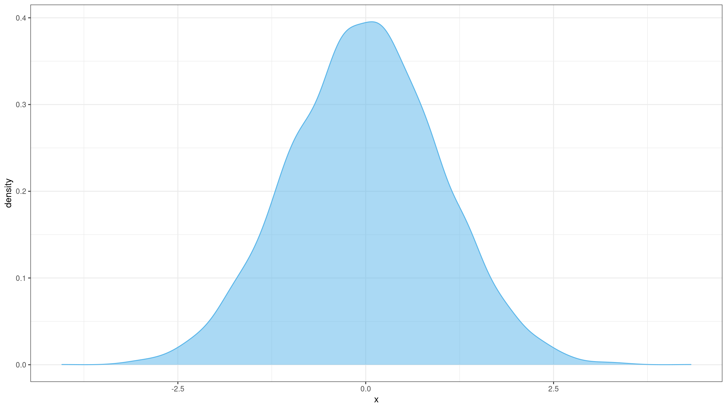
I have generated such a sample and evaluated its excess kurtosis. The excess kurtosis estimation was -0.01050842 (which is expected for $\mathcal{N}(0, 1)$). Next, I have added an outlier -1000. The “new” excess kurtosis value was 9794.628! Thus, a single extreme outlier could easily corrupt kurtosis estimation of a sample with thousands of “well-formed” elements.

However, if we recall that kurtosis is actually a measure of tailedness, such a change could be expected. Unfortunately, non-robustness leads to irreproducibility: we can’t rely on the kurtosis value from a single sample.

Here is a short R snippet that reproduces this experiment:

> library(e1071) # kurtosis from e1071 uses Joanes-Gill Type 3 approach (b2) by default
> set.seed(42)
> x <- rnorm(10000)
> kurtosis(x)
[1] -0.01050842
> kurtosis(c(-1000, x))
[1] 9794.628

Conclusion

In this post, we briefly covered some sources of kurtosis misleadingness. It’s too easy to get invalid insights about a distribution based on a standalone kurtosis value. If you still want to work with kurtosis, make sure that:

• You are sure that the underlying distribution is unimodal.
• You clearly understand the target kurtosis definition.
• If samples contain extreme outliers (e.g., the distribution is heavy-tailed), a non-robust kurtosis may be corrupted.

References

• [Joanes1998]
  Joanes, Derrick N., and Christine A. Gill. “Comparing measures of sample skewness and kurtosis.” Journal of the Royal Statistical Society: Series D (The Statistician) 47, no. 1 (1998): 183-189.
  https://doi.org/10.1111%2F1467-9884.00122
• [Bastianin2020]
  Bastianin, Andrea. “Robust measures of skewness and kurtosis for macroeconomic and financial time series.” Applied Economics 52, no. 7 (2020): 637-670.
  https://doi.org/10.1080/00036846.2019.1640862
• [Kim2004]
  Kim, Tae-Hwan, and Halbert White. “On more robust estimation of skewness and kurtosis.” Finance Research Letters 1, no. 1 (2004): 56-73.
  https://doi.org/10.1016/S1544-6123(03)00003-5
• [Moors1988]
  Moors, J. J. A. “A quantile alternative for kurtosis.” Journal of the Royal Statistical Society: Series D (The Statistician) 37, no. 1 (1988): 25-32.
  https://doi.org/10.2307/2348376
• [Hogg1972]
  Hogg, Robert V. “More light on the kurtosis and related statistics.” Journal of the American Statistical Association 67, no. 338 (1972): 422-424.
  https://doi.org/10.2307/2284397
• [Crow1967]
  Crow, Edwin L., and M. M. Siddiqui. “Robust estimation of location.” Journal of the American Statistical Association 62, no. 318 (1967): 353-389.