Misleading skewness

Skewness is a commonly used measure of the asymmetry of the probability distributions. A typical skewness interpretation comes down to an image like this:

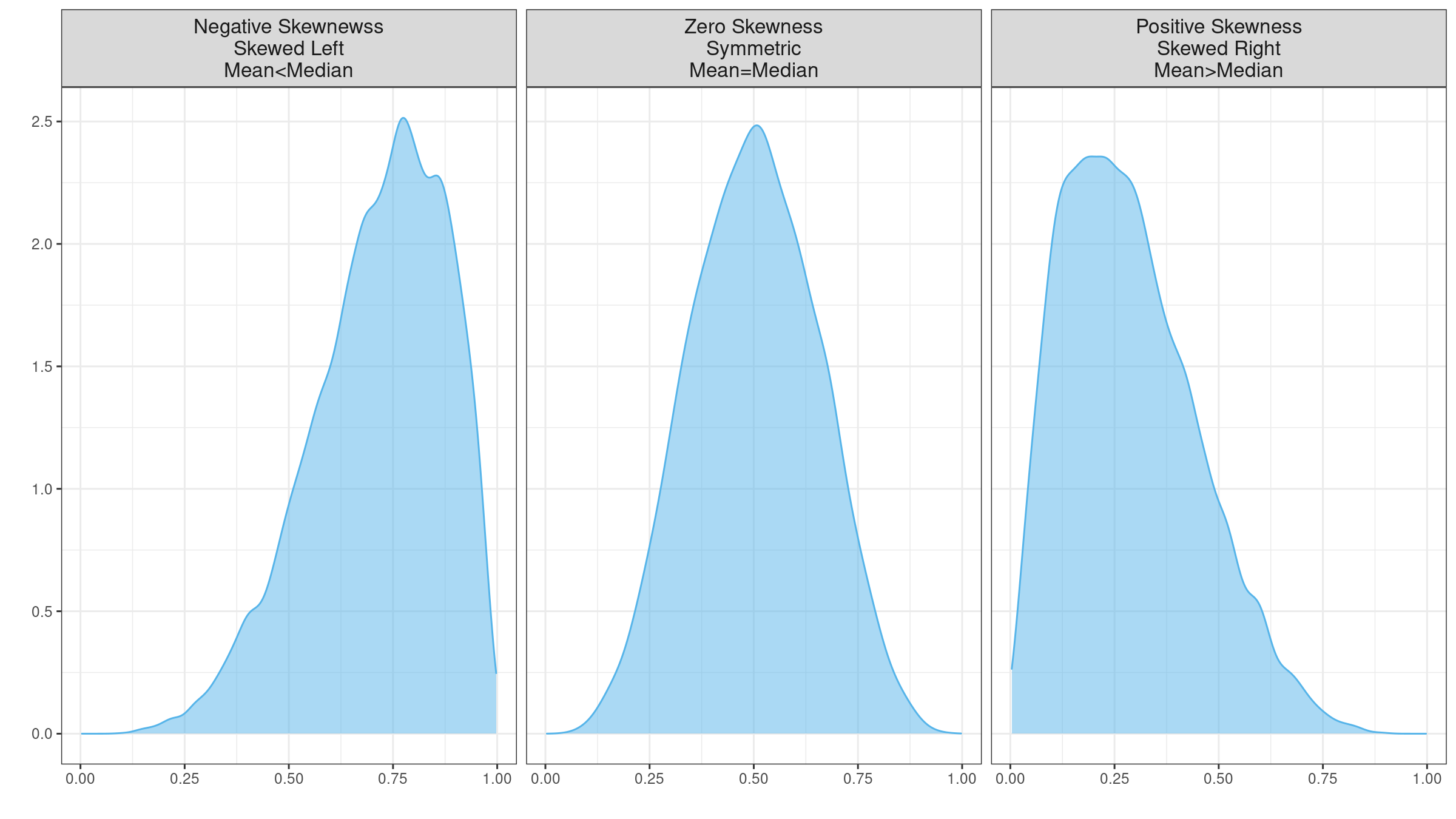
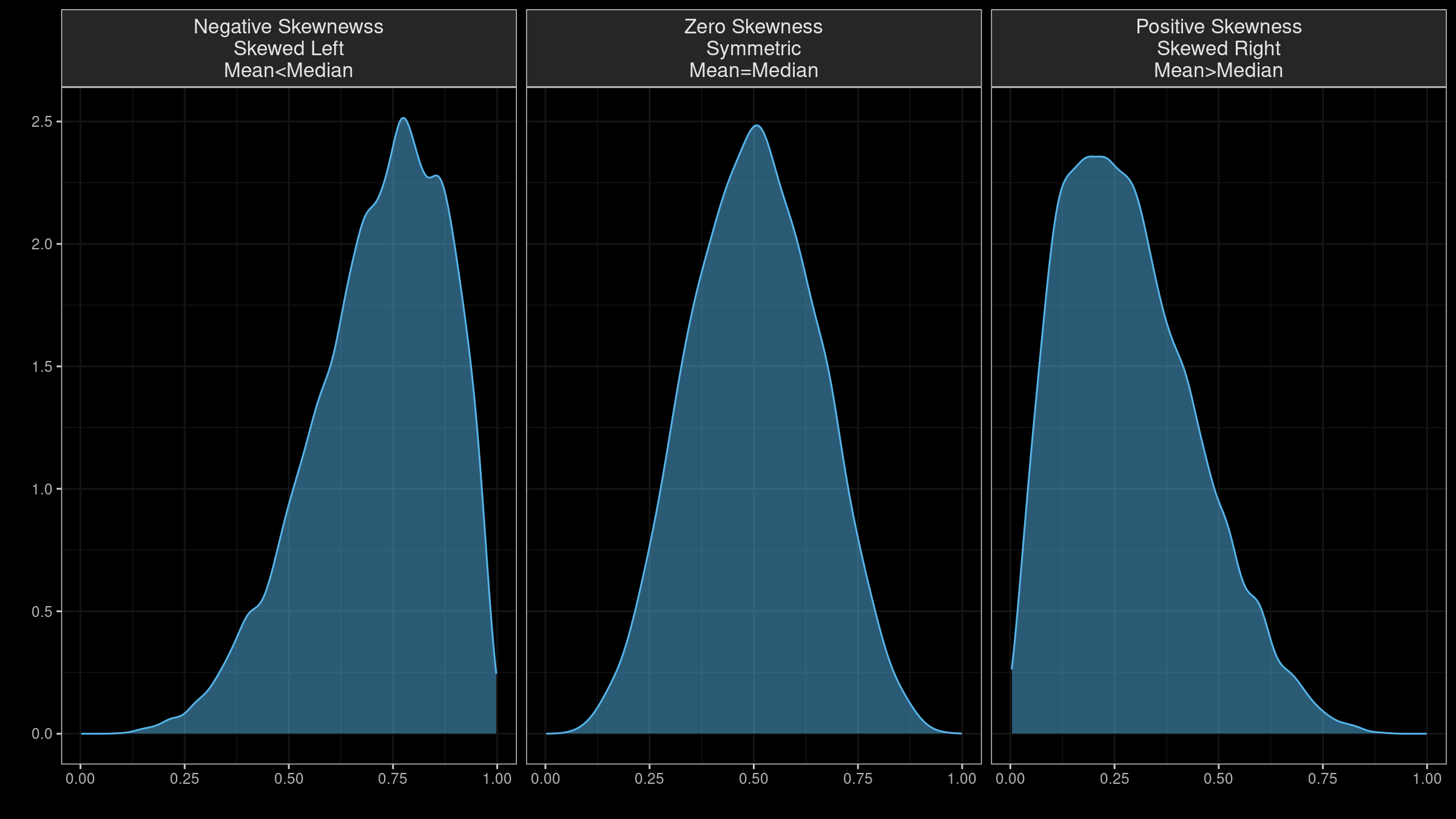
It looks extremely simple: using the skewness sign, we get an idea of the distribution form and the arrangement of the mean and the median. Unfortunately, it doesn’t always work as expected. Skewness estimation could be a highly misleading metric (even more misleading than the standard deviation). In this post, I discuss four sources of its misleadingness:

• “Skewness” is a generic term; it has multiple definitions. When a skewness value is presented, you can’t always guess the underlying equation without additional details.
• Skewness is “designed” for unimodal distributions; it’s meaningless in the case of multimodality.
• Most default skewness definitions are not robust: a single outlier could completely distort the skewness value.
• We can’t make conclusions about the locations of the mean and the median based on the skewness sign.

Multiple Definitions

Skewness is an ambiguous term. In general, it should be treated as a measure of the asymmetry, but different researchers use different ways to calculate the actual value. Let’s briefly discuss some of the most popular definitions. Hereinafter, we use the following notation:

• $x = \{ x_1, x_2, \ldots, x_n \}$: a sample of size $n$
• $\overline{x} = \sum x_i / n$: the sample mean
• $m_k = \frac{1}{n} \sum (x_i - \overline{x})^k$: the $k^\textrm{th}$ sample central moment
• $s^2 = \frac{1}{n-1} \sum (x_i - \overline{x})^2$: the unbiased sample variance
• $x_{\textrm{mode}}$: the mode
• $Q_p$: the $p^\textrm{th}$ quantile
• $x_m = Q_{0.5}$: the sample median

One of the most popular ways to express skewness is to use the third-moment equations. However, there are several kinds of corresponding formulas. The classic taxonomy with three common third-moment-based skewness definitions is described in [Joanes1998]:

However, the third-moment approach is not the only one that defines skewness. In the case of a unimodal distribution, we could also use the Pearson Mode Skewness (or Pearson’s first skewness coefficient).

The mode detection in the continuous case could be a challenging problem, so we could also use the Pearson Median Skewness (or Pearson’s second skewness coefficient):

Both approaches (the third-moment-based equations from the Joanes-Gill classification and Pearson’s coefficients) are not robust since they involve non-robust moments. As the robust alternative, we can use Bowley’s skewness (also known as quartile skewness coefficient or Yule’s coefficient):

This approach has a generalization by Groeneveld and Meeden:

Another popular robust measure of skewness is medcouple which is the median of the following function values:

for all pairs $(x_i, x_j)$ such that $x_i \geq x_m \geq x_j$ (if $x_i = x_m = x_j$, we assume $h(x_i, x_j) = \textrm{sign}(i+j-1-m)$).

The list goes on. The most important fact is that skewness has many different definitions. Without a context, it’s hard to tell which approach is used (typically, the best guess is a third-moment based skewness like $b_1$ or $g_1$).

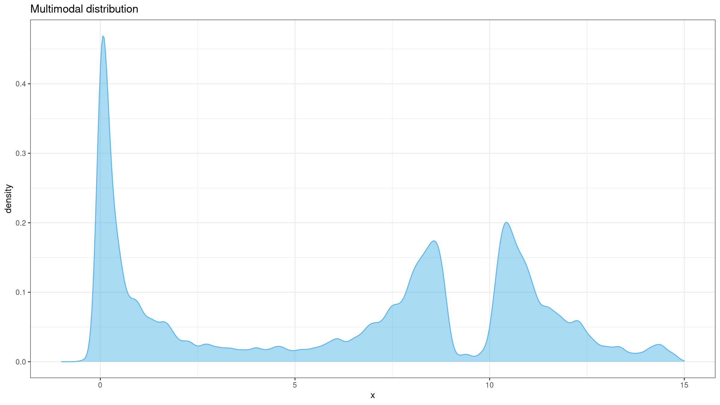
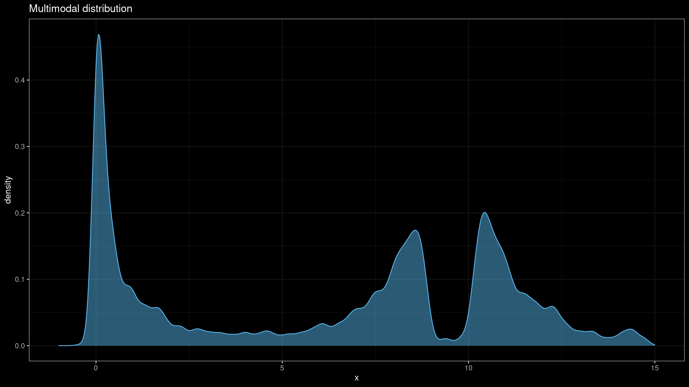
Multimodality

Regardless of the definition, skewness value is meaningful only for unimodal distributions. If the distribution has multiple modes, the raw skewness value will not help you to get any insights about the actual distribution form. Thus, it makes sense to check the distribution for unimodality first (e.g., using the lowland multimodality detector).

Non-robustness

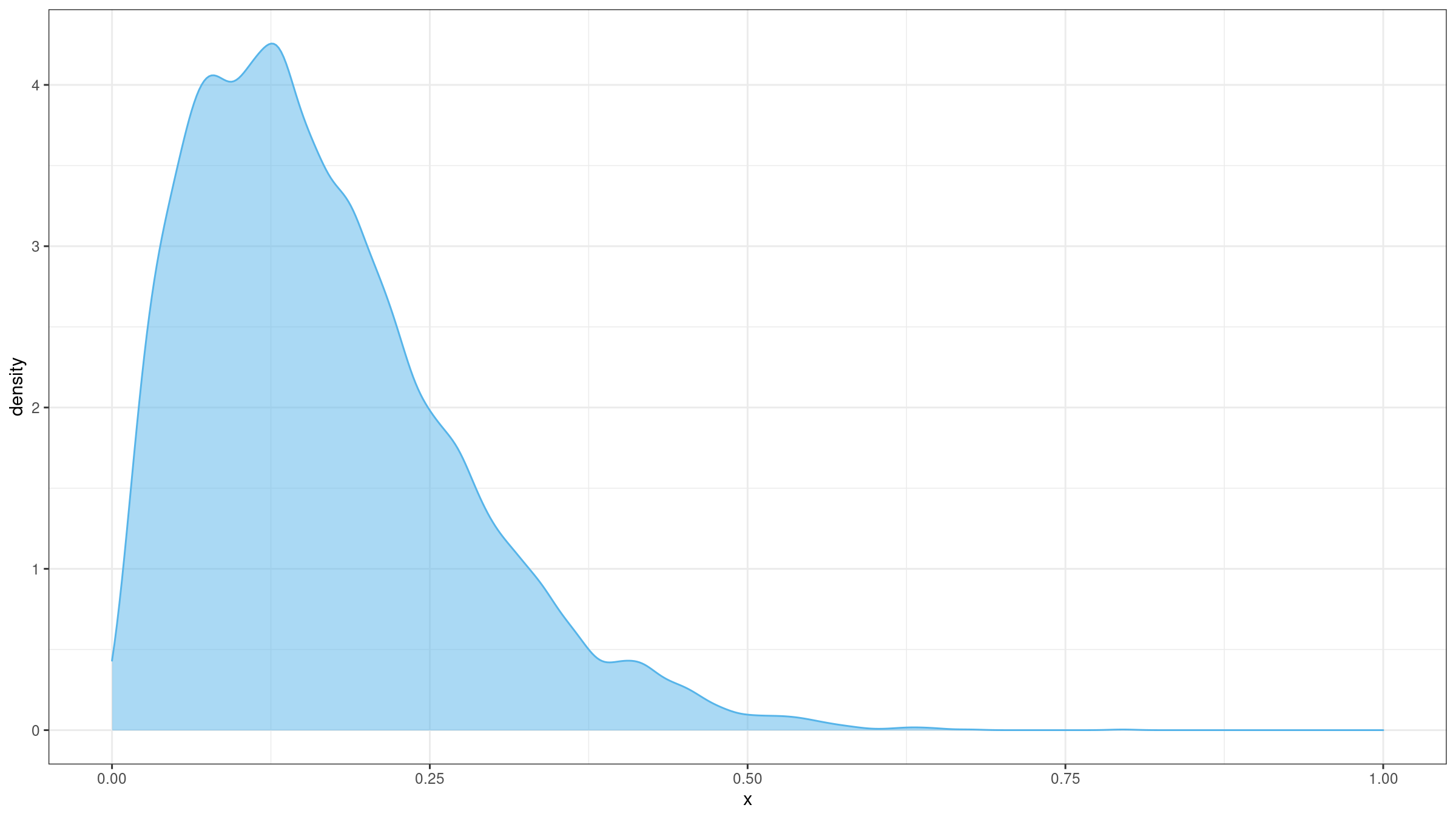
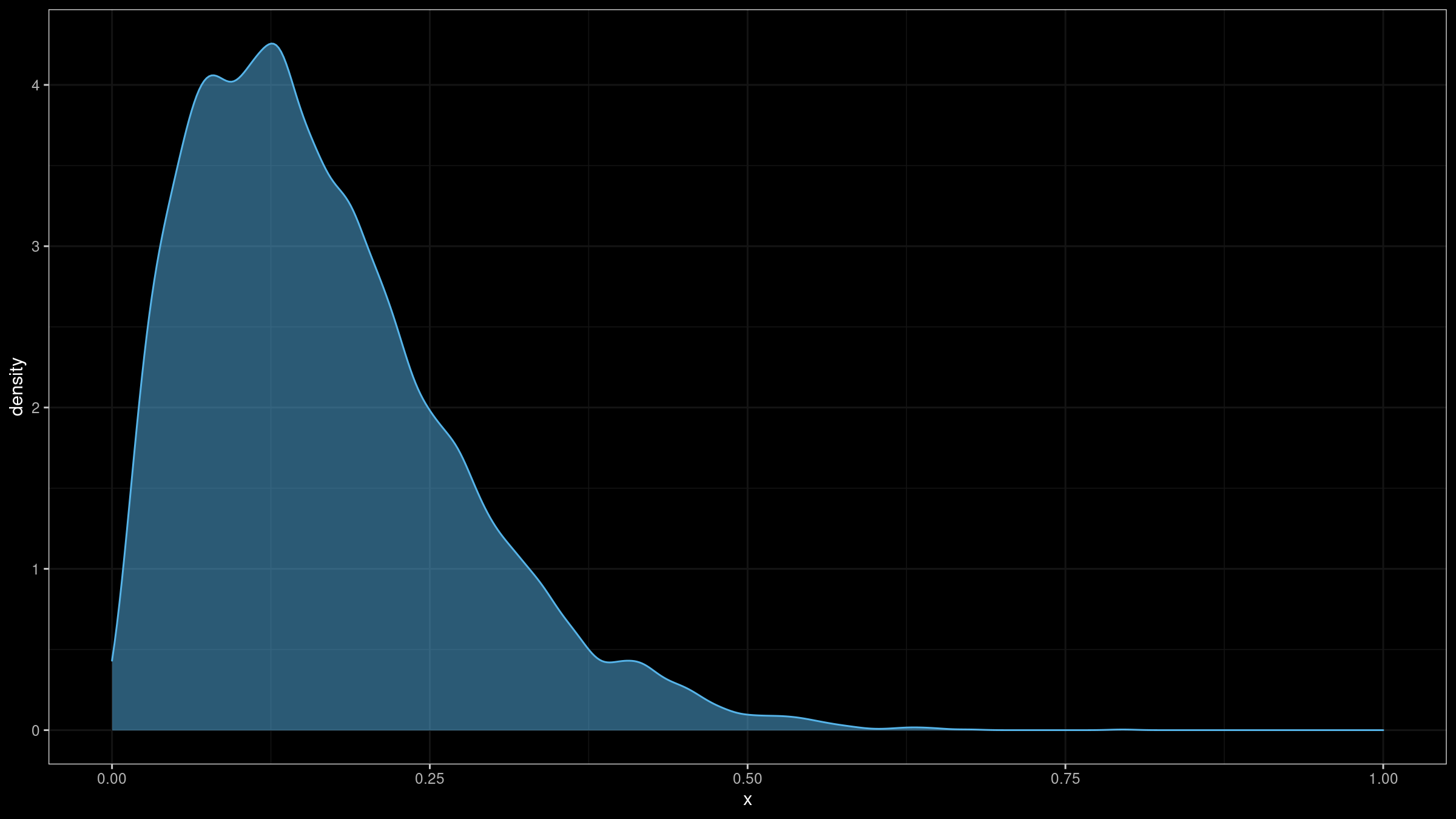
The classic third-moment skewness is not robust. This means that a single outlier could unpredictably corrupt the skewness value. Let’s illustrate the problem with an example. Imagine we build a sample with 10000 elements randomly taken from the Beta distribution $\textrm{Beta}(2, 10)$. The underlying distribution is right-skewed (the “true” distribution skewness is positive):

I have generated such a sample and evaluated its skewness. The skewness estimation was 0.9673111. Next, I have added an outlier -1000. The “new” skewness value was -99.95875! Thus, a single extreme outlier could easily corrupt skewness estimation of a sample with thousands of “well-formed” elements.

Here is a short R snippet that reproduces this experiment:

> library(e1071) # skewness from e1071 uses Joanes-Gill Type 3 approach (b1) by default
> set.seed(42)
> x <- rbeta(10000, 2, 10)
> skewness(x)
[1] 0.9673111
> skewness(c(-1000, x))
[1] -99.95875

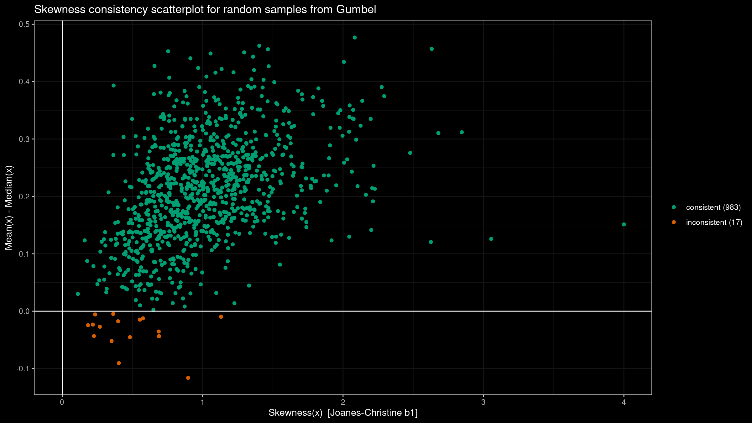
Breaking the Mean-Median rule

There is a well-known rule of thumb that says that the mean if left of the median for left-skewed distributions, and right of the median for right-skewed distributions. This empirical rule could work in some “simple” cases, but it doesn’t work in the general case.

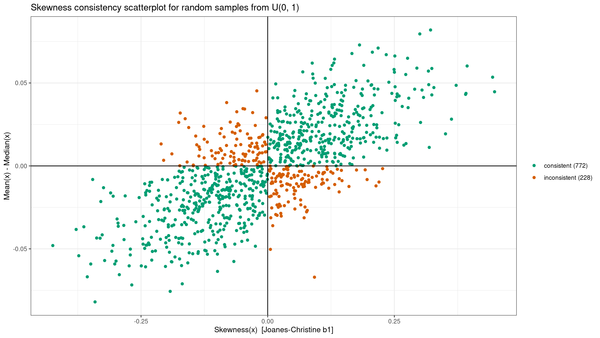
This problem is well-covered in [Hippel2005] where the author demonstrates multiple examples of the rule violations. In addition to this article, let’s perform our own experiment:

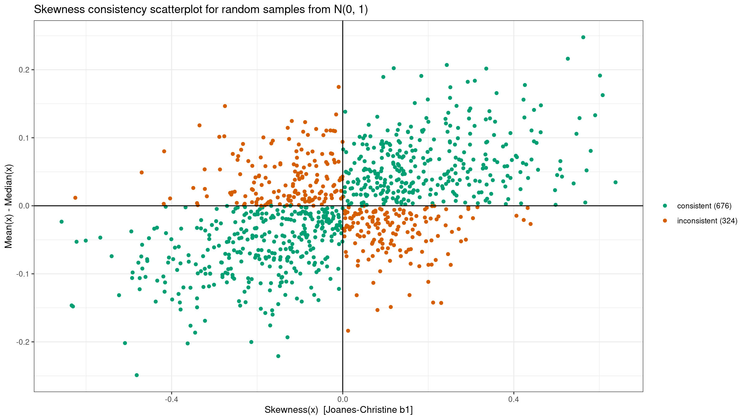
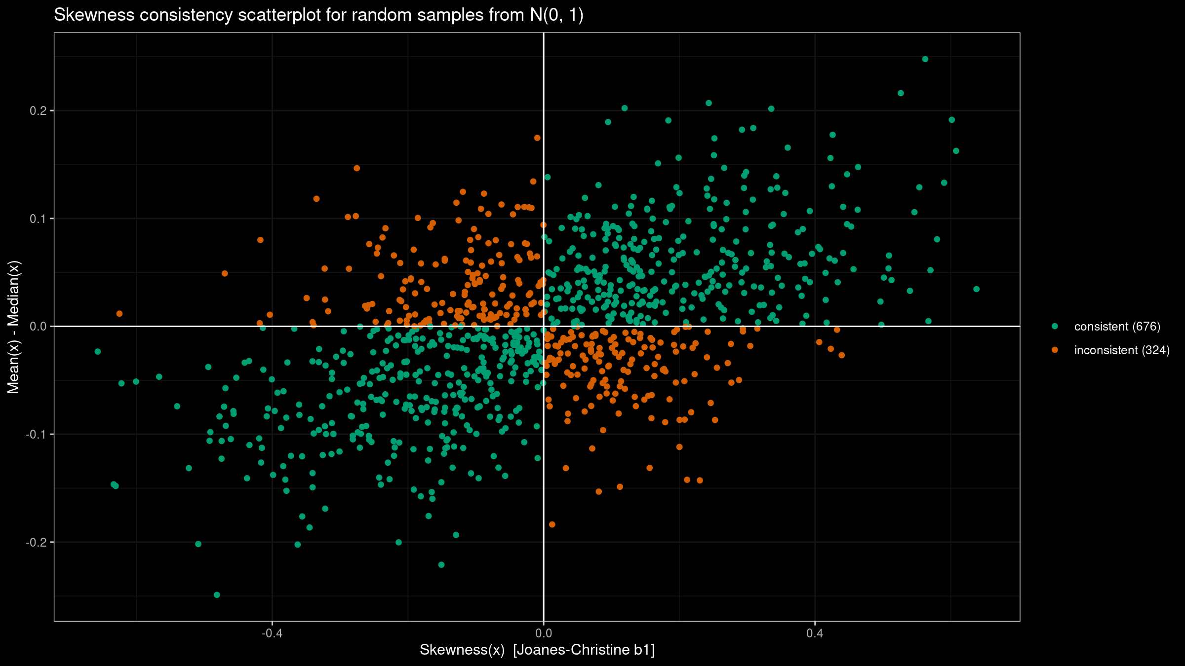
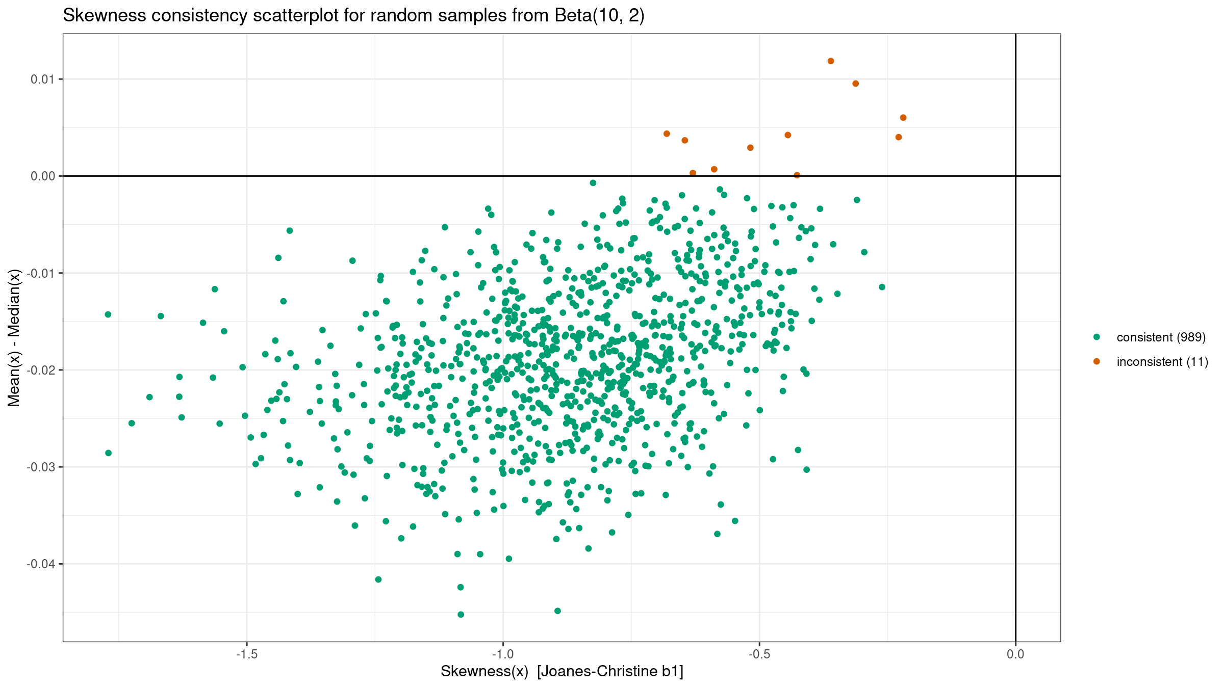
• Generate 1000 random samples of size 100 from the given distribution: the standard normal distribution N(0, 1), the standard uniform distribution U(0, 1), the left-skewed Beta distribution Beta(10, 2), and the right-skewed Gumbel distribution Gumbel.
• For each sample, we evaluate the third-moment-based skewness $b_1$ and the difference between the mean and the median. According to the rule of thumb, these values should have the same sign.
• Draw a scatterplot where we highlight “consistent” samples (the values actually have the same sign) and “inconsistent” samples (the values have different signs).

Here are the results:

Conclusion

In this post, we briefly covered some sources of skewness misleadingness. It’s too easy to get invalid insights about a distribution based on a skewness value. If we still want to work with skewness, make sure that:

• You are sure that the underlying distribution is unimodal.
• You clearly understand the target skewness definition.
• If samples contain extreme outliers (e.g., the distribution is heavy-tailed), a non-robust skewness may be corrupted.

References

• [Joanes1998]
  Joanes, Derrick N., and Christine A. Gill. “Comparing measures of sample skewness and kurtosis.” Journal of the Royal Statistical Society: Series D (The Statistician) 47, no. 1 (1998): 183-189.
  https://doi.org/10.1111%2F1467-9884.00122
• [Hippel2005]
  Von Hippel, Paul T. “Mean, median, and skew: Correcting a textbook rule.” Journal of statistics Education 13, no. 2 (2005).
  https://doi.org/10.1080/10691898.2005.11910556