Misleading standard deviation
The standard deviation may be an extremely misleading metric. Even minor deviations from normality could make it completely unreliable and deceiving. Let me demonstrate this problem using an example.
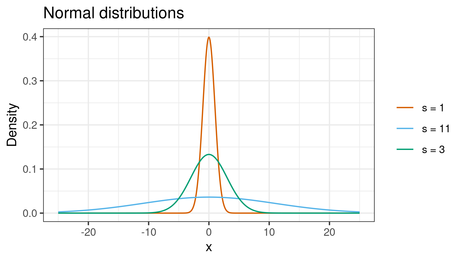
Below you can see three density plots of some distributions. Could you guess their standard deviations?
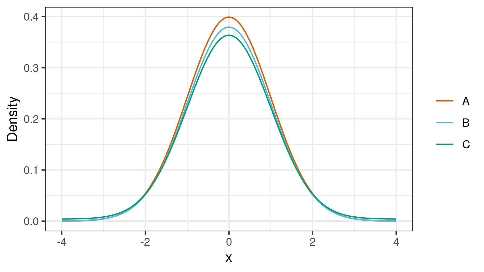
The correct answers are $1.0, 3.0, 11.0$. And here is a more challenging problem: could you match these values with the corresponding distributions?
All the density plots are close to each other, and all of them are similar to the normal distribution. How is this possible that one of them has $\sigma = 1.0$ and another one has $\sigma = 11.0$? The clue to this problem is the contaminated normal distributions that are mixtures of two normal distributions (see [Wilcox2017]). Let’s consider two normal distributions with zero mean values:
$$ X = \mathcal{N}(0, \sigma_x^2),\quad Y = \mathcal{N}(0, \sigma_y^2). $$We can build a new distribution $Z$ that is a mixture of $X$ (with weight $1-p$) and $Y$ (with weight $p$). Its standard deviation can be calculated as follows (a proof can be found here):
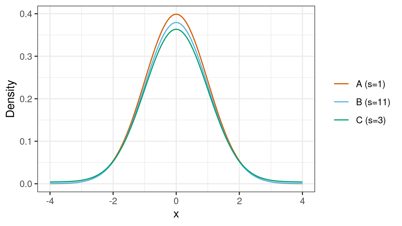
$$ \sigma_z = \sqrt{(1-p)\sigma_x^2 + p\sigma_y^2}. $$Now it’s time to reveal the actual distributions behind density plots from the picture:
- Distribution A is the standard normal distribution;
$\sigma_A = 1$. - Distribution B is the mixture of $\mathcal{N}(0, 1^2)$ (weight = 0.95) and $\mathcal{N}(0, 49^2)$ (weight = 0.05);
$\sigma_B = \sqrt{0.95\cdot 1^2 + 0.05\cdot 49^2} = \sqrt{121} = 11$ - Distribution C is the mixture of $\mathcal{N}(0, 1^2)$ (weight = 0.9) and $\mathcal{N}(0, 9^2)$ (weight = 0.1);
$\sigma_C = \sqrt{0.9\cdot 1^2 + 0.1\cdot 9^2} = \sqrt{9} = 3$
Let’s look at the corresponding density plots one more time:
Distributions B and C are extremely close to normal (we can evaluate the exact distance using the Kolmogorov-Smirnov distance or the Cramér–von Mises distance). However, $\sigma_B = 11$ and $\sigma_C = 3$. If we draw normal distributions based on such standard deviations, we get another picture that doesn’t look like the first picture at all!

When we describe samples using measures of dispersion, we should remember that the standard deviation is not a robust metric. This metric is too sensitive to the distribution tails and outliers. If we have small deviations from normality, the standard deviation becomes a misleading and dangerous way to describe the data. Note that all metrics based on the standard deviation like Cohen’s d and confidence intervals are also not robust.
If we work with data that may have slight deviations from normality (usually, all real data sets have such deviations), we can consider robust alternatives to the standard deviations as the median absolute deviation (MAD). You can find my other posts related to MAD here.
References
- [Wilcox2017]
Wilcox, Rand R. 2017. Introduction to Robust Estimation and Hypothesis Testing. 4th edition. Waltham, MA: Elsevier. ISBN 978-0-12-804733-0