Middle non-zero quantile absolute deviation

Median absolute deviation ($\operatorname{MAD}$) around the median is a popular robust measure of statistical dispersion. Unfortunately, if we work with discrete distributions, we could get zero $\operatorname{MAD}$ values. It could bring some problems if we use $\operatorname{MAD}$ as a denominator. Such a problem is also relevant to some other quantile-based measures of dispersion like interquartile range ($\operatorname{IQR}$).

This problem could be solved using the quantile absolute deviation around the median. However, it’s not always clear how to choose the right quantile to estimate. In this post, I’m going to suggest a choosing approach that is consistent with the classic $\operatorname{MAD}$ under continuous distributions (and samples without tied values).

Median absolute deviation and Quantile absolute deviations

Let $x = \{ x_1, x_2, \ldots, x_n \}$ be a sample from a mixture of a continues distribution and a discrete distribution. Let $Q(x, p)$ be an estimator of the $p^\textrm{th}$ quantile for sample $x$. In the scope of this post, we use the classic Hyndman-Fan Type 7 quantile estimator:

$$ Q(p) = x_{\lfloor h \rfloor}+(h-\lfloor h \rfloor)(x_{\lfloor h \rfloor+1})-x_{\lfloor h \rfloor}, \quad h = (n-1)p+1. $$

Using this notation, we could define the median absolute deviation around the median as follows:

$$ \operatorname{MAD}(x) = Q(|x - Q(x, 0.5)|, 0.5). $$

We could also define the quantile absolute deviation around a quantile as follows:

$$ \operatorname{QAD}(x, p, q) = Q(|x - Q(x, p)|, q). $$

Obviously, $\operatorname{MAD}$ is a special case of $\operatorname{QAD}$:

$$ \operatorname{MAD}(x) = \operatorname{QAD}(x, 0.5, 0.5). $$

Zero median absolute deviation

Let $k$ be the number of $x_i$ that equals exactly the median $Q(x, 0.5)$. If $k>n/2$, we have $\operatorname{MAD}(x) = 0$. For example, let’s consider the following sample:

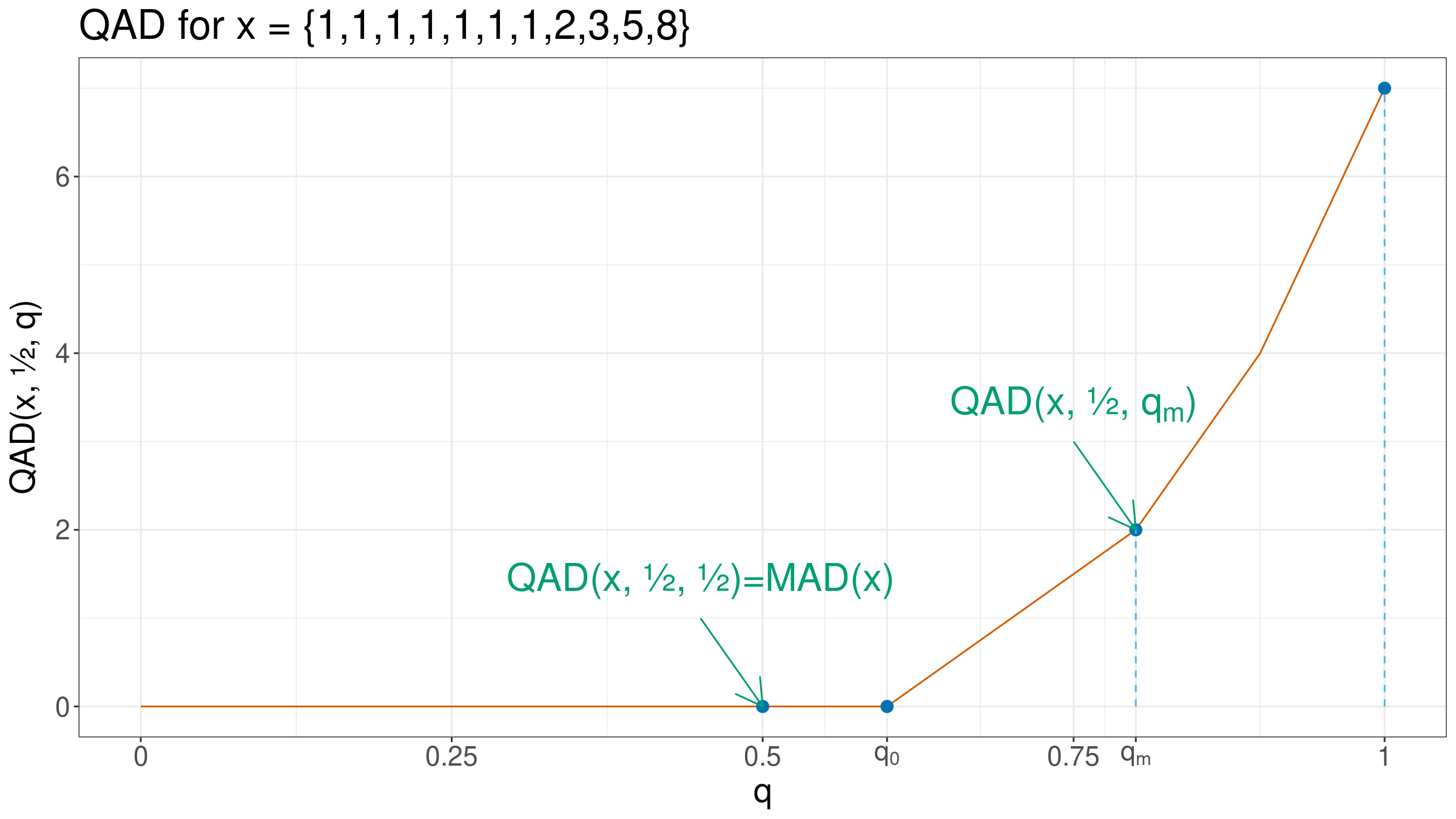
$$ x = \{ 1, 1, 1, 1, 1, 1, 1, 2, 3, 5, 8 \}. $$

The median value is $Q(x, 0.5) = 1$. And here is the list of absolute deviations:

$$ |x-Q(x, 0.5)| = \{ 0, 0, 0, 0, 0, 0, 0, 1, 2, 4, 7 \}. $$

It’s easy to see that the median absolute deviation is zero:

$$ \operatorname{MAD}(x) = \operatorname{QAD}(x, 0.5, 0.5) = 0. $$

Regardless of the $x_7, x_8, x_9, x_{10}, x_{11}$ values, $\operatorname{MAD}(x)$ will be still zero (while $k>n/2$ of the sample elements are the same).

Zero and non-zero quantile absolute deviation

Now let’s consider the quantile absolute deviation around the median:

$$ \operatorname{QAD}(x, 0.5, q) = Q(|x - Q(x, 0.5)|, q). $$

Since $|x - Q(x, 0.5)|$ is a sample with non-negative values that doesn’t depend on $q$, $\operatorname{QAD}(x, 0.5, q)$ is a monotonically non-decreasing function with non-negative values. Let’s say that $q_0 \in [0;1]$ is such a number that

$$ \begin{cases} \operatorname{QAD}(x, 0.5, q) = 0, &\textrm{for } q \leq q_0,\\ \operatorname{QAD}(x, 0.5, q) > 0, &\textrm{for } q > q_0. \end{cases} $$

In simple words, $q_0$ is the maximum value that gives us zero $\operatorname{QAD}$.

If sample $x$ contains exactly $k$ numbers that equal the median $Q(x, 0.5)$ and $n > 0$, it’s easy to see that

$$ q_0 = \frac{\max(k - 1, 0)}{n - 1}. $$

Thus, if $k > n /2$, we have $q_0 \geq 0.5$ so that $\operatorname{MAD}(x) = \operatorname{QAD}(x, 0.5, 0.5) = 0$.

Middle non-zero quantile absolute deviation around median

Zero $\operatorname{MAD}$ values could bring some problems if we use it as a denominator. It would be nice to have a robust measure of dispersion that never equals zero for samples with a non-zero range.

Let’s consider the midpoint between $q_0$ (the biggest quantile that provides zero $\operatorname{QAD}$) and $1$ (provides the maximum $\operatorname{QAD}$ value):

$$ q_m = \frac{q_0 + 1}{2}. $$

I suggest using $\operatorname{QAD}(x, 0.5, q_m)$ as a better measure of the statistical dispersion. Let’s call it the middle non-zero quantile absolute deviation:

$$ \operatorname{MNZQAD(x, 0.5)} = \operatorname{QAD(x, 0.5, q_m)}. $$

If a sample doesn’t contain tied elements, this metric is consistent with $\operatorname{MAD}$. Indeed, for $q_0=0$, we have

$$ \operatorname{QAD}(x, 0.5, q_m) = \operatorname{QAD}(x, 0.5, (q_0+1)/2) = \operatorname{QAD}(x, 0.5, 0.5) = \operatorname{MAD}(x). $$

With the help of consistency constants, we can also build a consistent estimator for the standard deviation under the normal distribution. Meanwhile, if a distribution is non-normal, $\operatorname{QAD}(x, 0.5, q_m)$ always gives non-zero values for samples with non-zero range ($\max(x)-\min(x) > 0$).

Middle non-zero quantile absolute deviation around quantile

We can also generalize $\operatorname{MNZQAD}$ and calculate this statistic for any quantile:

$$ \operatorname{MNZQAD(x, p)} = \operatorname{QAD(x, p, q_m)}, $$ $$ q_m = \frac{q_0 + 1}{2}, \quad q_0 = \frac{\max(k - 1, 0)}{n - 1}, \quad k = \sum_{i=1}^n \mathbf{1}_{Q(x, p)}(x_i), $$

where $\mathbf{1}$ is the indicator function:

$$ \mathbf{1}_U(u) = \begin{cases} 1 & \textrm{if}\quad u = U,\\ 0 & \textrm{if}\quad u \neq U. \end{cases} $$

Further notes about the suggested approach could be found here.