Analyzing distribution of Mono GC collections
Sometimes I want to understand the GC performance impact on an application quickly. I know that there are many powerful diagnostic tools and approaches, but I’m a fan of the “right tool for the job” idea. In simple cases, I prefer simple noninvasive approaches which provide a quick way to get an overview of the current situation (if everything is terrible, I always can switch to an advanced approach). Today I want to share with you my favorite way to quickly get statistics of GC pauses in Mono and generate nice plots like this:
Getting raw data
Mono has internal tools for getting brief data about GC events. You just should set a few environment variables:
export MONO_LOG_LEVEL=debug
export MONO_LOG_MASK=gc
As a result, we will get lines like follows in stdout:
Mono: GC_MINOR: (Nursery full) time 4.29ms, stw 4.51ms promoted 1337K major size: 5456K in use: 4785K los size: 8192K in use: 6821K
Mono: GC_MINOR: (Nursery full) time 2.55ms, stw 2.88ms promoted 558K major size: 6304K in use: 5528K los size: 8192K in use: 7039K
Mono: GC_MINOR: (Nursery full) time 6.70ms, stw 7.04ms promoted 2035K major size: 8512K in use: 7715K los size: 9216K in use: 7818K
Mono: GC_MAJOR: (LOS overflow) time 7.72ms, stw 8.02ms los size: 6144K in use: 2039K
Mono: GC_MAJOR_SWEEP: major size: 7936K in use: 5779K
Mono: GC_MINOR: (Nursery full) time 5.18ms, stw 5.43ms promoted 2420K major size: 10352K in use: 8351K los size: 6144K in use: 3150K
Mono: GC_MINOR: (Nursery full) time 5.81ms, stw 6.14ms promoted 1810K major size: 12192K in use: 10374K los size: 6144K in use: 3167K
Mono: GC_MINOR: (Nursery full) time 2.87ms, stw 3.21ms promoted 702K major size: 13056K in use: 11235K los size: 6144K in use: 3303K
Mono: GC_MINOR: (Nursery full) time 4.36ms, stw 4.71ms promoted 1028K major size: 14160K in use: 12374K los size: 6144K in use: 3320K
Mono: GC_MINOR: (Nursery full) time 3.25ms, stw 3.55ms promoted 708K major size: 14912K in use: 13157K los size: 6144K in use: 3320K
Mono: GC_MINOR: (Nursery full) time 3.34ms, stw 3.56ms promoted 908K major size: 16032K in use: 14189K los size: 6144K in use: 3447K
Mono: GC_MINOR: (Nursery full) time 2.77ms, stw 3.02ms promoted 614K major size: 16672K in use: 14894K los size: 6144K in use: 3467K
Mono: GC_MINOR: (Nursery full) time 5.00ms, stw 5.40ms promoted 918K major size: 17664K in use: 15878K los size: 6144K in use: 3549K
Mono: GC_MINOR: (Nursery full) time 4.01ms, stw 4.27ms promoted 1728K major size: 19584K in use: 17733K los size: 6144K in use: 3614K
Mono: GC_MINOR: (Nursery full) time 4.60ms, stw 4.84ms promoted 3514K major size: 23440K in use: 21511K los size: 6144K in use: 3655K
Mono: GC_MAJOR: (LOS overflow) time 18.97ms, stw 19.27ms los size: 6144K in use: 2346K
Mono: GC_MAJOR_SWEEP: major size: 25664K in use: 22669K
Mono: GC_MINOR: (Nursery full) time 3.88ms, stw 4.13ms promoted 1912K major size: 27472K in use: 24707K los size: 6144K in use: 2675K
Mono: GC_MINOR: (Nursery full) time 3.82ms, stw 4.14ms promoted 980K major size: 28448K in use: 25788K los size: 6144K in use: 3372K
Mono: GC_MINOR: (Nursery full) time 2.98ms, stw 3.24ms promoted 617K major size: 29040K in use: 26448K los size: 6144K in use: 3434K
Here we can find a lot of interesting information. However, it’s raw data, and it’s not easy to manually process such logs (especially if you have hundreds of lines). Let’s parse it and aggregate the most important data about GC pauses.
The script
I use the following simple regular expression for capturing most interesting lines: ^Mono: GC_(.{5}).*time ([0-9\\.]*)ms
(you can find an online version
here and
here).

Usually, I use R for simple statistics/plotting tasks.
Here is my script for processing such logs (assuming that we have the full log in output.txt):
library(ggplot2);library(dplyr);library(stringr)

lines <- readLines("output.txt")
df <- data.frame(str_match(lines, "^Mono: GC_(.{5}).*time ([0-9\\.]*)ms"))[,2:3]
colnames(df) <- c("type", "time")
df$time <- as.double(as.character(df$time))
df <- df %>% filter(type != "NA")

ggplot(df, aes(x=time, color=type)) +
  geom_histogram() +
  facet_grid(.~type, scales = "free")
ggsave("plot.png")

summary(df %>% filter(type == "MINOR"))
summary(df %>% filter(type == "MAJOR"))
Case study
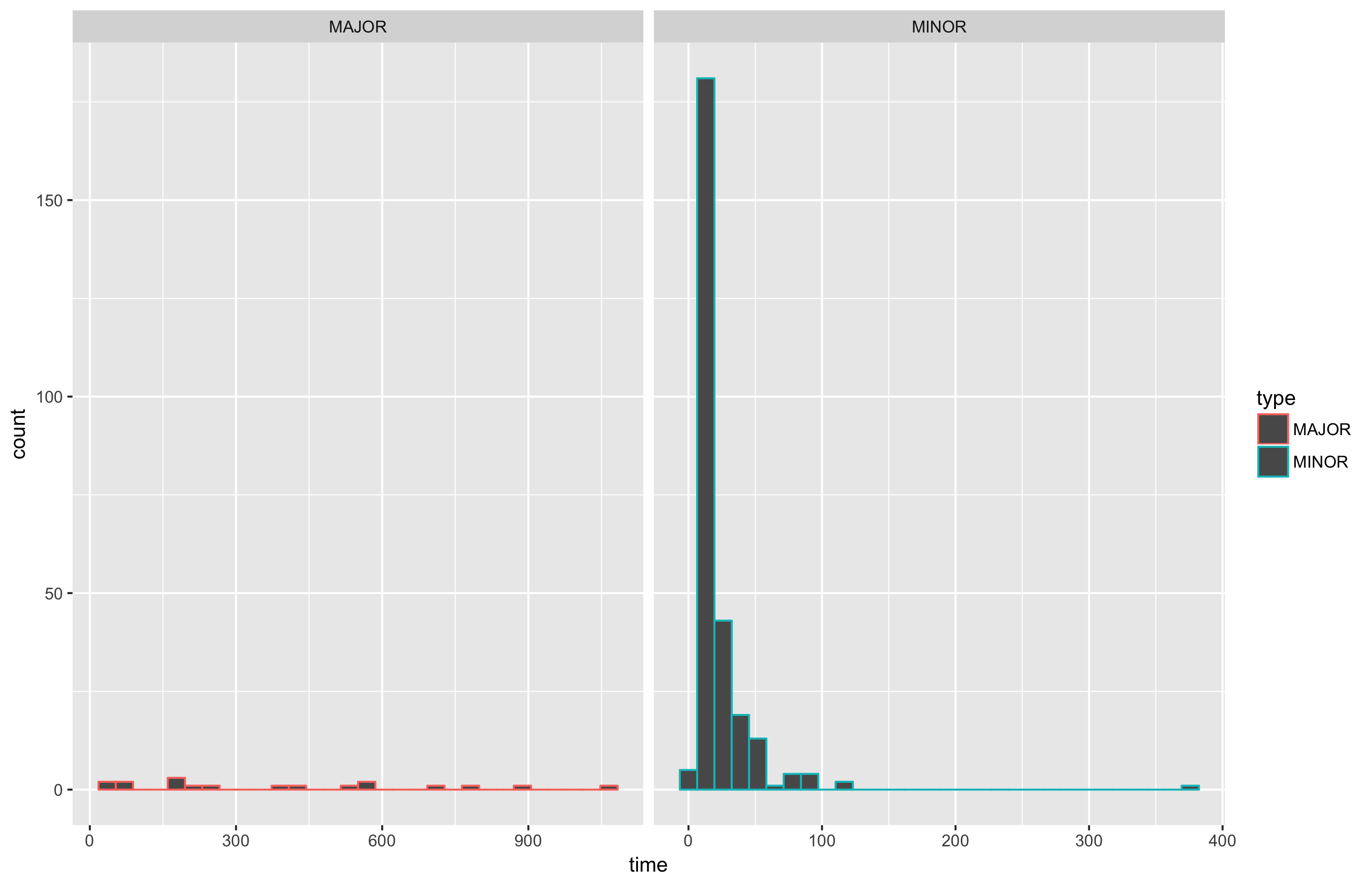
Once, I decided to play with the nursery-size value in Rider.
The default value is 4 MB, but it’s not the optimal value for Rider.
Let’s open a simple solution in Rider and look at the statistics.
nursery-size=4m
> summary(df %>% filter(type == "MINOR"))
    type           time
 MAJOR:   0   Min.   : 0.320
 MINOR:2029   1st Qu.: 6.990
              Median : 8.670
              Mean   : 8.664
              3rd Qu.: 9.910
              Max.   :84.190

> summary(df %>% filter(type == "MAJOR"))
    type         time
 MAJOR:20   Min.   :  68.16
 MINOR: 0   1st Qu.: 168.90
            Median : 237.40
            Mean   : 339.33
            3rd Qu.: 402.62
            Max.   :1068.22
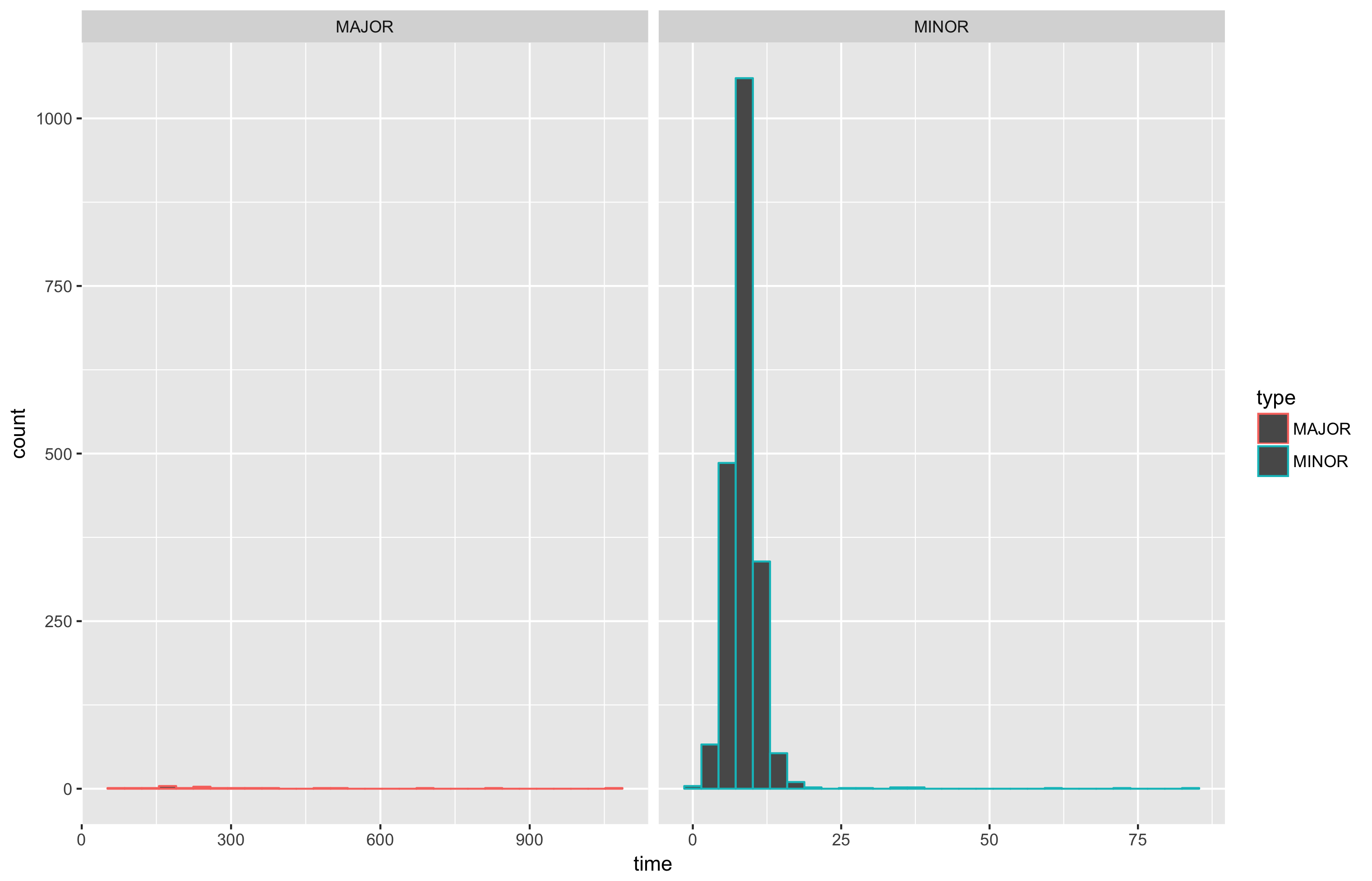
nursery-size=64m
> summary(df %>% filter(type == "MINOR"))
    type          time
 MAJOR:  0   Min.   :  3.42
 MINOR:273   1st Qu.: 11.72
             Median : 15.01
             Mean   : 22.72
             3rd Qu.: 20.79
             Max.   :379.26

> summary(df %>% filter(type == "MAJOR"))
    type         time
 MAJOR:18   Min.   :  22.94
 MINOR: 0   1st Qu.: 176.00
            Median : 317.68
            Mean   : 397.17
            3rd Qu.: 567.48
            Max.   :1052.87
The average time of GC_MINOR is bigger for 64 M (22.72ms vs. 8.664ms),
but the amount of GC_MINOR collections is 273 instead of 2029!
Performance impact
Does it really affect the performance? Let’s find out! I checked a subset of the Rider solution (212 projects) on Ubuntu 16.04. I measured the startup time (the time before solution is fully loaded include the full product initialization). I have analyzed the full distributions, but let’s look only at average numbers for simplification. The results:
Mono 4.8
nursery-size=4m      -> Time = ~75sec
nursery-size=64m     -> Time = ~47sec

Mono 5.2
nursery-size=4m      -> Time = ~95sec
nursery-size=64m     -> Time = ~40sec
After many additional checks on different solutions,
the nursery size was changed to 64 MB in Rider 2017.2,
it improved the startup experience for Linux and macOS users on huge solutions.
Default way to get statistics
You can also run mono with the --stats arguments and get a lot of useful information includes a report about GC.
It looks like follows:
GC statistics
Collection max time                 : 79.32 ms
Minor fragment clear                : 0.01 ms
Minor pinning                       : 6.78 ms
Minor scan remembered set           : 124.51 ms
Minor scan major blocks             : 47.46 ms
Minor scan los                      : 67.16 ms
Minor scan pinned                   : 0.01 ms
Minor scan roots                    : 14.70 ms
Minor fragment creation             : 1.38 ms
Major fragment clear                : 0.12 ms
Major pinning                       : 12.85 ms
Major scan pinned                   : 0.01 ms
Major scan roots                    : 128.16 ms
Major scan mod union blocks         : 48.61 ms
Major scan mod union los            : 4.63 ms
Major finish gray stack             : 190.74 ms
Major free big objects              : 0.00 ms
Major LOS sweep                     : 6.57 ms
Major sweep                         : 0.08 ms
Major fragment creation             : 0.56 ms
Number of pinned objects            : 11933
World stop                          : 7.60 ms
World restart                       : 2.77 ms

## workers finished                  : 14

Memgov alloc                        : 190944712
Memgov max alloc                    : 318818244
Minor GC collections                : 14
Major GC collections                : 10
Minor GC time                       : 420.70 ms
Major GC time                       : 434.76 ms
Major GC time concurrent            : 757.94 ms
It’s also a very useful trick, but I prefer to look at the distribution, so I typically collect full information about all GC collections.
Conclusion
When you start a performance investigation, you don’t know the current runtime characteristics in advance. These characteristics can be useful for initial hypotheses. It’s great when you can collect some high-level data without additional tools. I like to start with a quick and dirty checks which allow me to get a first impression about the current situation.
Of course, you usually need advanced profiling tools for full performance investigations.
And you should use it at the end for verifying your hypotheses and making final conclusions.
But it’s not always should be the first step because it takes too much time.
Also profilers are typically invasive tools,
the default Mono log profiler has huge overhead.
MONO_LOG_LEVEL=debug is a non invasive approach with low overhead,
you need only ten seconds for the setup and
you can run it on a customer computer without additional tools.
Data can be processed with a small R script which can be easily modified
if you want to calculate some advanced statistics.