Confusing tie correction in the classic Mann-Whitney U test implementation
In this post, we discuss the classic implementation of the Mann-Whitney U test for cases in which the considered samples contain tied values. This approach is used the same way in all the popular statistical packages.
Unfortunately, in some situations, this approach produces confusing p-values, which may be surprising for researchers
who do not have a deep understanding of ties correction.
Moreover, some statistical textbooks argue against the validity of the default tie correction.
The controversialness and counterintuitiveness of this approach may become a severe issue which may lead
to incorrect experiment design and flawed result interpretation.
In order to prevent such problems, it is essential to clearly understand
the actual impact of tied observations on the true p-value and
the impact of tie correction on the approximated p-value estimation.
In this post, we discuss the tie correction for the Mann-Whitney U test
and review examples that illustrate potential problems.
We also provide examples of the Mann-Whitney U test implementations from popular statistical packages:
wilcox.test from stats (R),
mannwhitneyu from SciPy (Python), and
MannWhitneyUTest from HypothesisTests (Julia).
At the end of the post, we discuss how to avoid possible problems related to the tie correction.
The importance of tie analysis
In the realm of mathematical statistics, we often work with random samples from continuous distributions. A common assumption made in this context is that the probability of encountering tied values is zero. While this statement holds true in an abstract theoretical world, issues arise during the transition to real-world data analysis.
In reality, the resolution of measurement devices is limited, and achieving infinite precision is virtually impossible. Consequently, the probability of ties in an actual realization of a random sample does not remain zero. The likelihood of ties in a dataset increases as the range of values narrows, and the sample size grows.
It is crucial to consider how tied values will be addressed when designing a statistical procedure for data analysis. Neglecting this aspect can lead to the failure of the statistical procedure or results that are significantly distorted. Some speculations on this topic can be found in various statistical textbooks:
A common assumption in the development of nonparametric procedures is that the underlying population(s) is (are) continuous. This assumption implies that the probability of obtaining tied observations is zero. Nevertheless, tied observations do occur in practice. These ties may arise when the underlying population is not continuous. They may even arise if the continuity assumption is valid. We simply may be unable, owing to inaccuracies in measurement, to distinguish between two very close observations (temperatures, lengths, etc.) that emanate from a continuous population.
— Hollander, M., Wolfe, D. A., & Chicken, E. (2013). Nonparametric Statistical Methods (3rd ed.). Wiley. Page 7.
Our hypotheses have been concerned with observations from continuous d.f. ’s, and this implies that the probability of any pair of observations being precisely equal (a so-called tie) is zero and that we may therefore neglect the possibility. Thus we have throughout this chapter assumed that observations could be ordered without ties, so that the rank-order statistics were uniquely defined. However, in practice, observations are always rounded off to a few significant figures, and ties will therefore sometimes occur.
— M. G. Kendall & Alan Stuart - The Advanced Theory of Statistics, Vol. II, 3rd Edition (2010, Wiley). Page 508.
The Mann-Whitney test assumes that the scores represent a distribution which has underlying continuity. With very precise measurement of a variable which has underlying continuity, the probability of a tie is zero. However, with the relatively crude measures which we typically employ in behavioral scientific research, ties may well occur. We assume that the two observations which obtain tied scores are really different, but that this difference is simply too refined or minute for detection by our crude measures.
— Sidney Siegel - Nonparametric statistics for the behavioral sciences (1956, McGraw-Hill). Page 124.
The Mann-Whitney U test
We consider the one-sided Mann-Whitney U test that compares two samples $\mathbf{x}$ and $\mathbf{y}$:
$$ \mathbf{x} = \{ x_1, x_2, \ldots, x_n \}, \quad \mathbf{y} = \{ y_1, y_2, \ldots, y_m \}. $$For the one-sided version, the alternative hypothesis states that $\mathbb{P}(X > Y) > \mathbb{P}(Y > X)$. The core concept of this test suggests calculating the U statistic:
$$ U(x, y) = \sum_{i=1}^n \sum_{j=1}^m S(x_i, y_j),\quad
S(a,b) = \begin{cases} 1, & \text{if } a > b, \ 0.5, & \text{if } a = b, \ 0, & \text{if } a < b. \end{cases} $$
It is a simple rank-based statistic, which varies from $0$ to $nm$. Once we get the value of $U$, we should match it with the distribution of $U$ statistics under the valid null hypothesis. There are several approaches to doing this. When the sample sizes are small, and there are no tied values, we can calculate the exact p-value using dynamic programming to obtain the exact probability of obtaining the given $U$ statistic for the given $n$ and $m$. However, this approach does not support tied values, and it is impractical for large samples due to its computational complexity. Another popular way to implement the Mann-Whitney U test is to approximate the U statistic distribution by the normal distribution $\mathcal{N}(\mu_U, \sigma^2_U)$, where
$$ \mu_U = \frac{nm}{2},\quad \sigma_U = \sqrt{\frac{nm(n+m+1)}{12}}. $$Tie correction for the Mann-Whitney U test
In the case of ties, it is suggested to adjust $\sigma_U$. A typical recommendation for such a correction looks like this:
$$ \sigma_{U,\textrm{ties}} = \sqrt{\frac{nm}{12} \left( n+m+1 - \frac{\Sigma_{k=1}^{K} (t_k^3 - t_k)}{(n+m)(n+m-1)} \right)}, $$where $t_k$ is “the number of ties for the $k^\textrm{th}$ rank,” assuming ranks in the combined sample $\{ x_1, x_2, \ldots, x_n, y_1, y_2, \ldots, y_m \}$. Note that this accounts not only for between-sample ties (e.g., $x_1=y_1$), but also for within-sample ties (e.g., $x_1=x_2$ or $y_1=y_2$). This approach is advocated in multiple classic textbooks like “Nonparametric Statistical Methods” (1973) by M. Hollander, D.A. Wolfe and “Statistical methods based on ranks” (1975) by E.L. Lehmann, H. J. M. D’Abrera.
A case study
The tie correction may be counterintuitive in some cases. Let us illustrate the problem using the following pair of samples of size 10:
$$ \mathbf{x}_A = \{ 7.5, 7.6, 7.7, 7.8, 7.9, 8.0, 8.1, 8.2, 8.3, 8.4 \}, $$$$ \mathbf{y}_A = \{ 5.5, 5.6, 5.7, 5.8, 5.9, 6.0, 6.1, 6.2, 6.3, 6.4 \}. $$Here we have the extreme case (see Mann-Whitney U Test: Minimum meaningful statistical levelMann-Whitney U Test: Minimum meaningful statistical level) of the Mann-Whitney U test:
the samples do not overlap.
Therefore, the expected exact p-value is $1 / C_{20}^{10} \approx 5.4 \cdot 10^{-6}$.
However, the normal approximation without tie correction described above
gives another expected p-value of $\approx 9.1 \cdot 10^{-5}$
(it noticeably differs from the exact p-value,
which is another severe issue (see When R's Mann-Whitney U test returns extremely distorted p-values
By Andrey Akinshin
·
2023-04-25
Discussing corner cases in which wilcox.test returns distorted p-valuesWhen R's Mann-Whitney U test returns extremely distorted p-values).
Now imagine that we reduce the resolution of our measurement device and get rounded versions of $\mathbf{x}_A$ and $\mathbf{y}_A$:
$$ \mathbf{x}_B = \operatorname{round}(\mathbf{x}_A) = \{ 8, 8, 8, 8, 8, 8, 8, 8, 8, 8 \}, $$$$ \mathbf{y}_B = \operatorname{round}(\mathbf{y}_A) = \{ 6, 6, 6, 6, 6, 6, 6, 6, 6, 6 \}. $$The pair $(\mathbf{x}_B, \mathbf{y}_B)$ is not so different from the pair $(\mathbf{x}_A, \mathbf{y}_A)$
in the context of comparison.
Both cases represent the same data up to the rounding precision.
Also, both cases represent the extreme case of the Mann-Whitney U test,
in which the samples of size $10$ do not overlap.
Therefore, we may expect the same p-value for both cases.
Now let us review the actual output of the Mann-Whitney U test using various popular statistical packages.
We consider the approximate implementation of the Mann-Whitney U test via
wilcox.test from stats (R),
mannwhitneyu
from SciPy (Python), and
MannWhitneyUTest
from HypothesisTests (Julia).
xA <- c(7.5, 7.6, 7.7, 7.8, 7.9, 8.0, 8.1, 8.2, 8.3, 8.4)
yA <- c(5.5, 5.6, 5.7, 5.8, 5.9, 6.0, 6.1, 6.2, 6.3, 6.4)
xB <- round(xA)
yB <- round(yA)

wilcox.test(xA, yA, alternative = "greater", exact = F)$p.value

## 9.13359e-05

wilcox.test(xB, yB, alternative = "greater", exact = F)$p.value

## 7.968956e-06
import numpy as np
from scipy.stats import mannwhitneyu

xA = np.array([7.5, 7.6, 7.7, 7.8, 7.9, 8.0, 8.1, 8.2, 8.3, 8.4])
yA = np.array([5.5, 5.6, 5.7, 5.8, 5.9, 6.0, 6.1, 6.2, 6.3, 6.4])
xB = np.round(xA)
yB = np.round(yA)

print(mannwhitneyu(xA, yA, alternative="greater", method="asymptotic").pvalue)

## 9.133589555477501e-05

print(mannwhitneyu(xB, yB, alternative="greater", method="asymptotic").pvalue)

## 7.968955844033122e-06
using HypothesisTests
using Statistics

xA = [7.5, 7.6, 7.7, 7.8, 7.9, 8.0, 8.1, 8.2, 8.3, 8.4]
yA = [5.5, 5.6, 5.7, 5.8, 5.9, 6.0, 6.1, 6.2, 6.3, 6.4]
xB = round.(xA)
yB = round.(yA)

pvalue(ApproximateMannWhitneyUTest(xA, yA), tail=:right)

## 9.133589555477498e-5

pvalue(ApproximateMannWhitneyUTest(xB, yB), tail=:right)

## 7.968955844033115e-6
All three functions provide consistent results. For the pair $(\mathbf{x}_A, \mathbf{y}_A)$, we always have the expected p-value of $\approx 9.1 \cdot 10^{-5}$. However, for the pair $(\mathbf{x}_B, \mathbf{y}_B)$, the returned p-value is $\approx 8 \cdot 10^{-6}$. This result is 11.5 times smaller than the expected one!
Understanding the tie correction
In the above example, the difference between results may look like a bug in the implementation. However, it is actually expected that rounding leads to changes in p-values. To better understand this phenomenon, we review how rounding affects the distribution of the $U$ statistic values. For simplicity, let us consider two following distributions:
$$ F = \mathcal{U}(0, 2), \quad G = \lfloor \mathcal{U}(0, 2) \rfloor. $$Distribution $F$ is a uniform distribution on $[0;2]$, which is a continuous one and which (theoretically) does not produce tied observations. Distribution $G$ is a floored version of $F$, which is essentially the “fair” Bernoulli distribution with $p=0.5$ (it produces $0$ and $1$ with equal probability, like for the fair coin flip). We also reduce the sample sizes to $n=m=2$.
Next, we run a numerical simulation for $F$ and $G$. In this simulation, we generate multiple sample pairs $x$ and $y$ of size $2$ from the given distribution, calculate the value of the $U$ statistic, and build the corresponding sample values. Here are the results:
| U | 0 | 1 | 2 | 3 | 4 |
|---|---|---|---|---|---|
| F | 0.16(6) | 0.16(6) | 0.33(3) | 0.16(6) | 0.16(6) |
| G | 0.063 | 0.250 | 0.374 | 0.250 | 0.063 |
And here are the corresponding histograms:
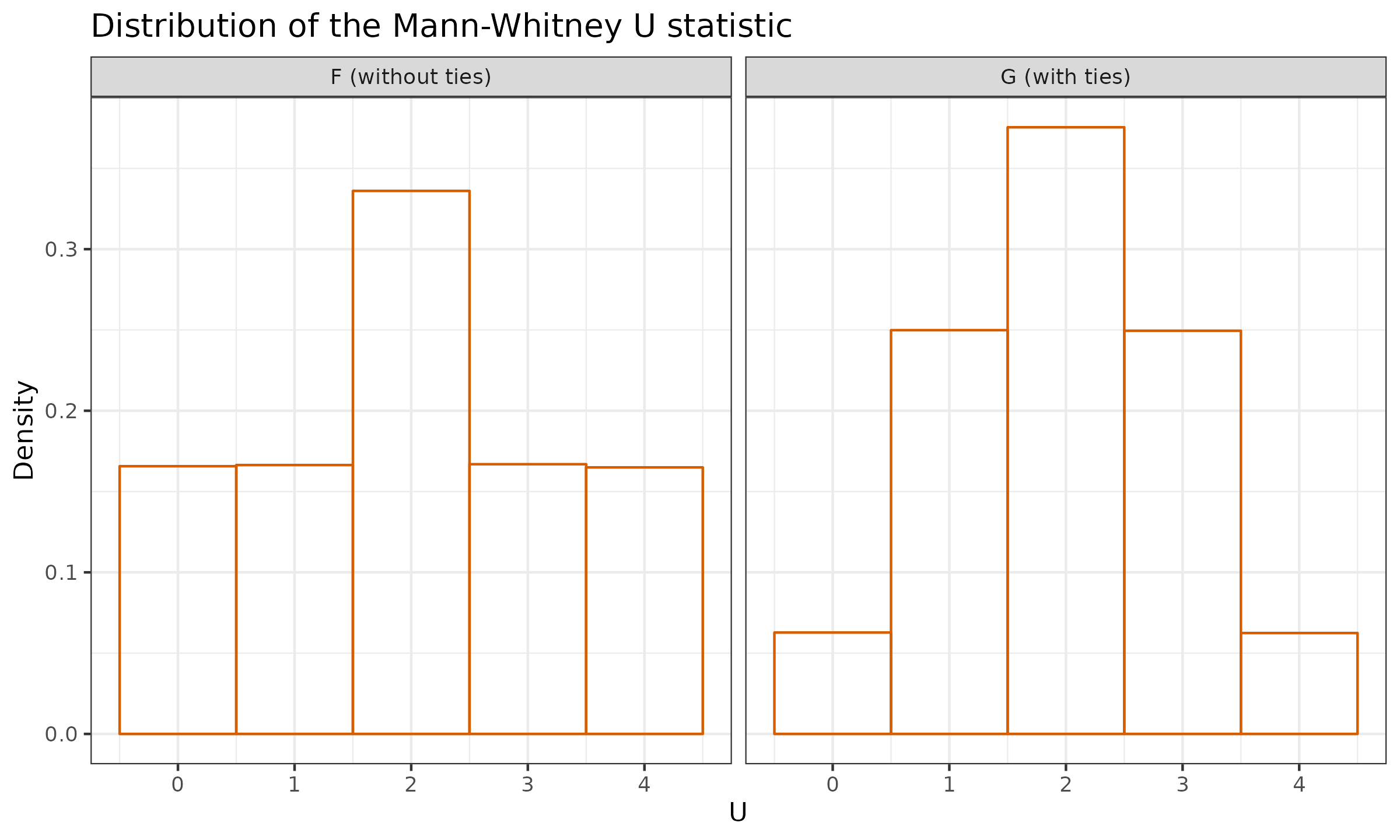
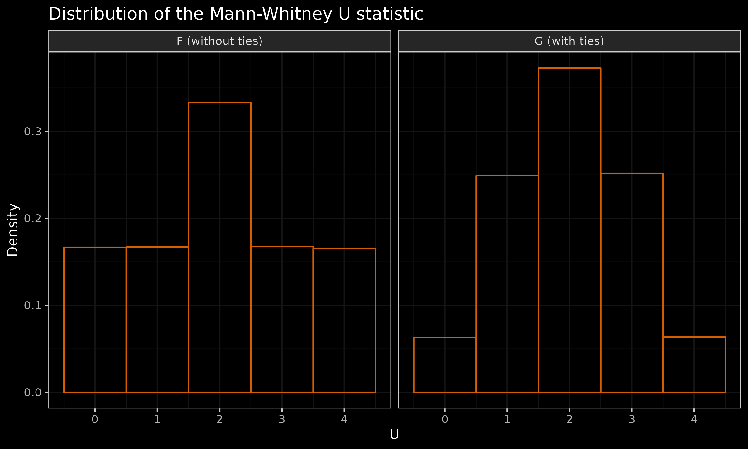
As we can see, the transition from $F$ to $G$ (which is rounding) changes the actual distribution of the $U$ statistic. After rounding, the maximum value of $U$ becomes more extreme: the probability of $U=4$ decreases from $\approx 0.167$ to $\approx 0.063$. Therefore, we can’t apply the non-tied p-values estimators (both the exact one and the approximated one) to $G$ distribution. This happens because we lose some information during rounding. Indeed, let us consider the following pair of samples:
$$ \mathbf{x}_A = \{ 1.3, 1.2 \},\quad \mathbf{y}_A = \{ 1.1, 0.1 \}. $$For this situation, we have $U_A = 4$. Now we consider a rounded version of this pair:
$$ \mathbf{x}_B = \{ 1, 1 \},\quad \mathbf{y}_B = \{ 1, 0 \}. $$For the rounded case, we have $U_B = 3$, which is not extreme anymore. Therefore, the rounding changes the obtained $U$ value for a huge class of changes. As a result, the probability of obtaining $U=4$ decreases: this event becomes more extreme.
Controversialness of the tie correction
When we have between-sample ties (e.g., $x_1=y_1$), the need for the p-value adjustment looks reasonable. Indeed, if the underlying distribution is truly continuous and the true ties cannot exist, the loss of information is obvious. With infinite precision, we would get either $x_1 < y_1$ or $x_1 > y_1$, but getting $x_1=y_1$ implies that we have less information about the data. This limits our ability to speculate about the true difference between the underlying distribution.
The impact of within-sample ties (e.g., $x_1=x_2$) is more confusing since it doesn’t affect the obtained value of the $U$ statistic. If we have only within-sample ties, and we know that these are “false” ties (since the underlying distribution is continuous and the “true” ties are impossible), why should we make any adjustments? To understand the tie correction for within-sample ties, we should recall that the p-value describes the “unusualness” of the results with the assumption that the null hypothesis is true. If the null hypothesis is actually true and both $x$ and $y$ come from the same distribution, we should not distinguish between-sample ties and within-sample ties, right? Here is one more quote that emphasizes the importance of accounting for within-sample ties:
In certain situations involving tied observations there arises an ambiguity that is not always resolved correctly. Suppose that the treatment observations are 6, 6, 6, 9 and the control observations 1, 3, 4, 10, with large values of $W_s$ being significant. Since ties occur only among the treatment observations, no question arises concerning the value of $W_s$. The treatment ranks are 4, 5, 6, 7 and the rank sum $W_s$ thus has the value 22. It is now tempting to compute the significance probability as in Sec. 2 or obtain it from Table B to be 12/70 = .1714. On the other hand, the approach of the present section gives $W_s^* = 22$ and the significance probability 11/70 = .1571 [Prob. 45(i)]. Which of these two values is correct?
Recalling the basis for such probability calculations, we see that the actual observations must be compared with all possible ways of assigning the eight numbers 1, 3, 4, 6, 6, 6, 9, 10 to treatment and control. Many of these will split the three tied observations, assigning some to one group and some to the other, and in these cases the value of $W_s$ is not defined. Hence, there is no validity in the first approach, and the correct value of the significance probability is .1571.
— Lehmann, Erich Leo, and H. J. M. D’Abrera. “Statistical methods based on ranks.” Nonparametrics. San Francisco, CA, Holden-Day (1975). Page 20 (Section 4 “The treatment of ties”)
While these arguments seem reasonable, the extreme case (non-overlapped samples with within-sample ties and without between-sample) still looks confusing. Since the within-sample ties do not affect the $U$ statistic value, and they are not “true” ties, why do we make the adjustments? I’m not the only person who is confused by this situation. I have found the following quotes that advocate against acknowledging the within-sample ties (emphasis is mine):
If the ties occur between two or more observations in the same group, the value of U is not affected. But if ties occur between two or more observations involving both groups, the value of U is affected. Although the effect is usually negligible, a correction for ties is available for use with the normal curve approximation which we employ for large sample.
— Sidney Siegel, Nonparametric statistics for the behavioral sciences (1956, McGraw-Hill), page 124
When ties occur only within the first or within the second group, they do not affect the outcome of the large-sample approximation. However, when there is at least one observation in the first group and at least one from the second that share a common rank, the asymptotic version of the WMW procedure is rendered too conservative. A correction for ties reduces the value of the denominator of the z statistic, and so renders the outcome of the WMW procedure less conservative (i.e., gives smaller p values) (Siegel and Castellan 1988).
— Bergmann, Reinhard, John Ludbrook, and Will P. J. M. Spooren. “Different Outcomes of the Wilcoxon-Mann-Whitney Test from Different Statistics Packages.” The American Statistician 54, no. 1 (February 2000): 72. https://doi.org/10.2307/2685616, page 73
These arguments also seem reasonable. But how do we separate the within-sample ties from the between-sample ties? Indeed, let us consider the following pair of samples:
$$ \mathbf{x} = \{ 0, 0, 0, 2 \},\quad \mathbf{y} = \{ 0, 0, 1 \}. $$Here we have a group of five tied zeros: three in $x$ and two in $y$. The tie correction equation requires us to provide the total number of tied values in the group. If we want to ignore the within-sample ties, how should we apply the tie correction for such a case?
Inaccuracies of the tie correction
The tie correction has one more problem. While it slightly improves the accuracy of the calculation, it doesn’t always provide reliable results:
A normal approximation is again available when m and n are not too small and the maximum proportion of observations tied at any value is not too close to 1.
— Lehmann, Erich Leo, and H. J. M. D’Abrera. “Statistical methods based on ranks.” Nonparametrics. San Francisco, CA, Holden-Day (1975). Page 20 (Section 4 “The treatment of ties”)
Let us illustrate this problem with one more example:
$$ F = \mathcal{U}(0, 1.05), \quad G = \lfloor \mathcal{U}(0, 1.05) \rfloor. $$A random value from distribution $G$ is $0$ with probability $20/21$ and $1$ with probability $1/21$, so the “average” proportion of tied values is quite close to $1$. Let us generate multiple samples of size $n=m=10$ from these distributions. Here are the corresponding histograms:
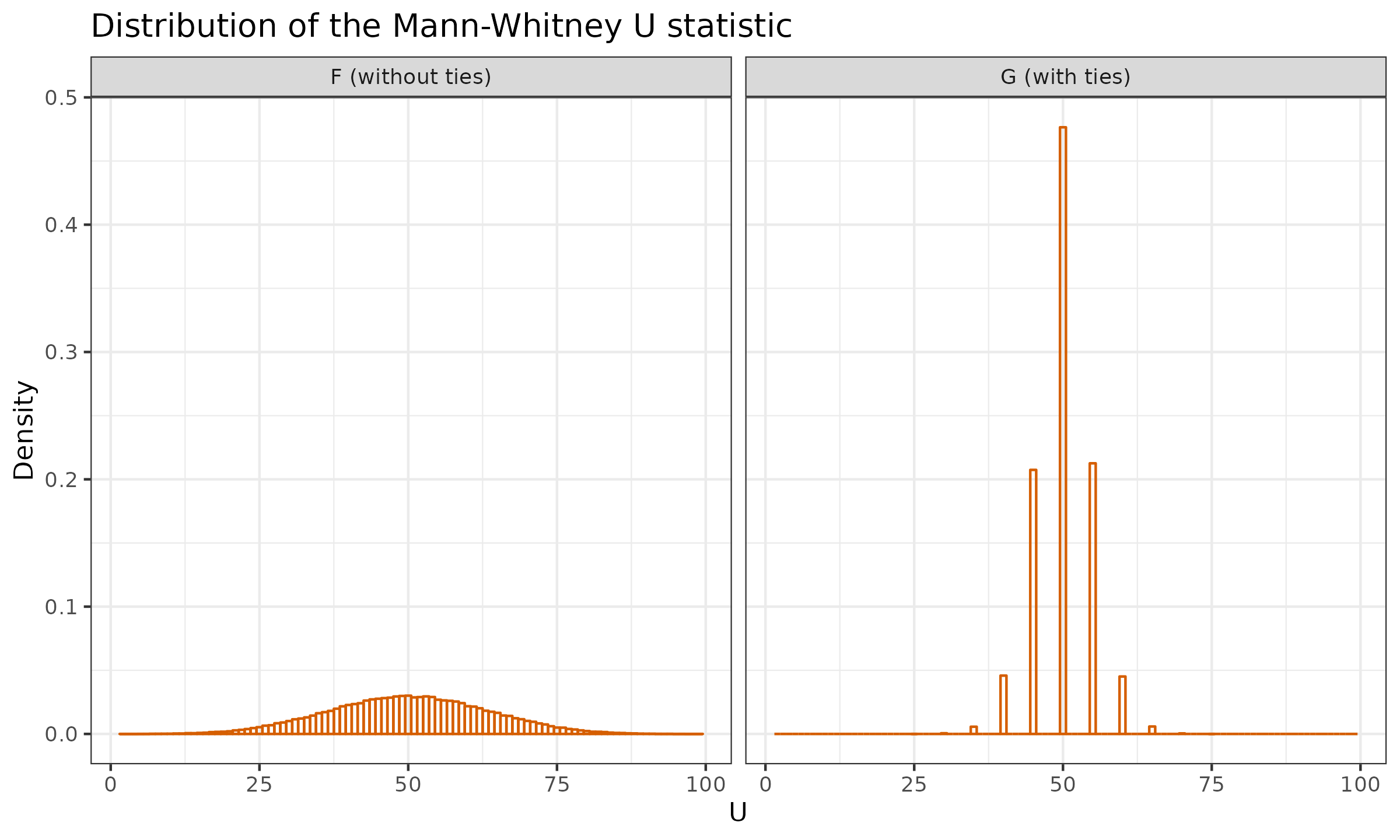
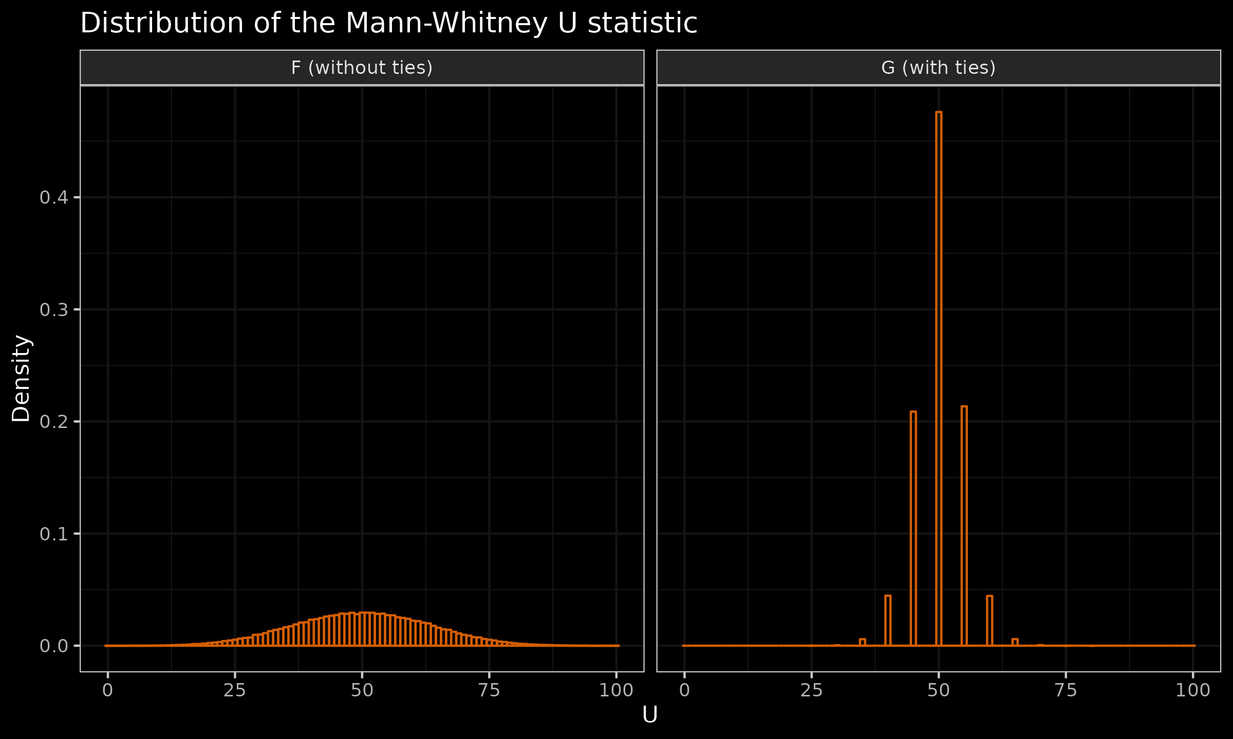
Now let us focus on distribution $G$. According to the simulation results, we have:
$$ \mathbb{P}(U_F \geq 55) \approx 0.368,\quad \mathbb{P}(U_G \geq 55) \approx 0.264. $$Now let us review a pair of samples for which $U=55$:
$$ \mathbf{x} = \{ 1, 0, 0, 0, 0, 0, 0, 0, 0, 0 \},\quad \mathbf{y} = \{ 0, 0, 0, 0, 0, 0, 0, 0, 0, 0 \}. $$Here is the Mann-Whitney U test result based on the normal approximation with the default tie correction:
wilcox.test(c(1, 0, 0, 0, 0, 0, 0, 0, 0, 0),
            c(0, 0, 0, 0, 0, 0, 0, 0, 0, 0),
            alternative = "greater")$p.value

## cannot compute exact p-value with ties
The obtained p-value of $\approx 0.184$ is quite inaccurate. As we can see, the default tie correction is too aggressive: the observed p-value is noticeably less than the expected value of $\approx 0.264$.
Thus, we have the following picture:
- If the number of ties is small, the tie correction for the normal approximation doesn’t produce a noticeable result on the p-value.
- If the number of ties is huge, the tie correction for the normal approximation is highly inaccurate.
Hence, the actual usefulness of the default tie correction is questionable.
Avoiding tie correction
Summarizing the above reasonings, the default tie correction doesn’t work well in some cases. I believe that it is possible to come up with a better tie correction equation that acknowledges not only the total number of tied observations in the same group $t_k$, but also the exact numbers of tied values in the current group that come from $\mathbf{x}$ and $\mathbf{y}$ independently. However, I would like to suggest another approach.
The best way to avoid problems with tie correction is to avoid situations in which we should apply the tie correction. I’m not a fan of testing the nil hypothesis that states the difference between distributions is exactly zero. Instead, I advocate using tests that check that the true difference between distributions is larger than a reasonably chosen threshold (so-called practical significance tests, minimum-effect tests, equivalence tests, etc.). With such an approach, we can define the minimum effect size of interest $\delta$ as half of the resolution interval (or higher if needed). To apply such a test, we should use the classic Mann-Whitney U test for samples $\mathbf{x}-\delta$ and $\mathbf{y}$. In this case, the between-sample tied values will be practically impossible. If the underlying distribution is supposed to be continuous, all the within-sample tied values are “false” ties and can be ignored. As a result, no ties correction is needed.