Nonparametric Cohen's d-consistent effect size

Andrey Akinshin · 2020-06-25

Update: the second part of this post is available here.

The effect size is a common way to describe a difference between two distributions. When these distributions are normal, one of the most popular approaches to express the effect size is Cohen’s d. Unfortunately, it doesn’t work great for non-normal distributions.

In this post, I will show a robust Cohen’s d-consistent effect size formula for nonparametric distributions.

Cohen’s d

Let’s start with the basics. For two samples $X = {X_{1}, X_{2}, \dots, X_{n_{X}}}$ and $Y = {Y_{1}, Y_{2}, \dots, Y_{n_{Y}}}$ , the Cohen’s d is defined as follows ([Cohen1988]):

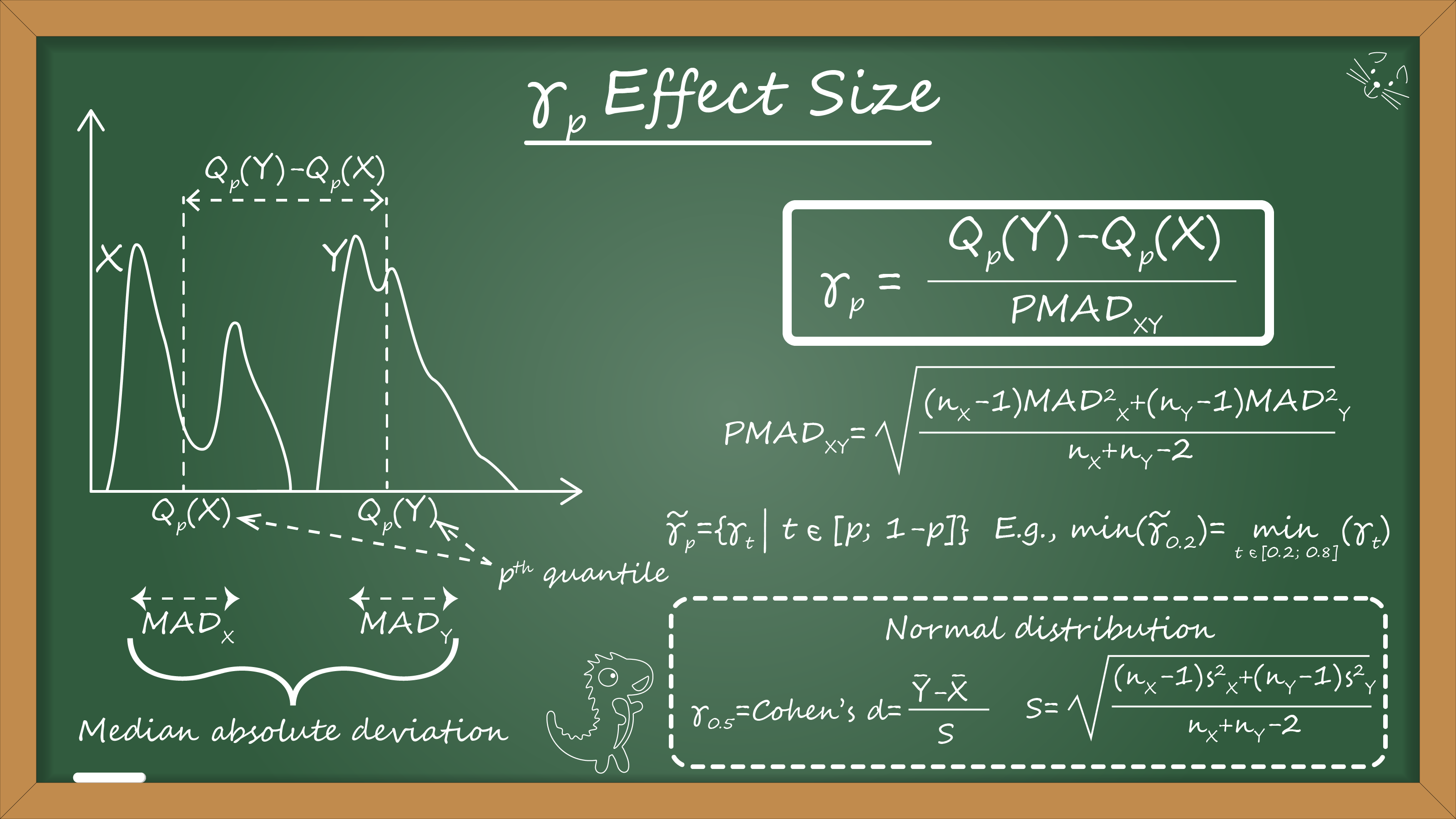
d = \frac{\overset{―}{Y} - \overset{―}{X}}{s}

where $s$ is the pooled standard deviation:

s = \sqrt{\frac{(n_{X} - 1) s_{X}^{2} + (n_{Y} - 1) s_{Y}^{2}}{n_{X} + n_{Y} - 2}} .

Our goal is to build a robust effect size formula that works the same way for normal distributions, but also is applicable for nonparametric distributions.

Existing nonparametric effect size measures

There are some existing nonparametric effect size measures, but most of them are clamped (they have fixed lower and upper bounds):

Cliff’s Delta ( Dominance statistics: Ordinal analyses to answer ordinal questions
By Cliff N · 1993 cliff1993): $[- 1; 1]$
Vargha-Delaney A ( A Critique and Improvement of the "CL" Common Language Effect Size Statistics of McGraw and Wong
By András Vargha, Harold D Delaney, Andras Vargha · 2000 vargha2000): $[0; 1]$
Wilcox’s Q ( A Robust Nonparametric Measure of Effect Size Based on an Analog of Cohen's d, Plus Inferences About the Median of the Typical Difference
By Rand Wilcox · 2019 wilcox2019): $[0; 1]$

Let’s consider the two following cases of nonoverlapped distribution pairs:

X^{(1)} \in [0; 5] vs. Y^{(1)} \in [10; 20]

and

X^{(2)} \in [0; 5] vs. Y^{(2)} \in [50; 100] .

In both cases, all of the above measures have extreme values. Thus, they don’t help to distinguish these cases. Meanwhile, the effect for $X^{(2)} vs. Y^{(2)}$ is much larger than the effect for $X^{(1)} vs. Y^{(1)}$ . It would be nice to have an effect size measure that highlights this difference.

Quantiles and the shift function

When we compare two nonparametric distributions, it’s a good idea to track differences for all quantile values. We can do it via the shift function ( Empirical Probability Plots and Statistical Inference for Nonlinear Models in the Two-Sample Case
By Kjell Doksum · 1974 doksum1974, Plotting with confidence – Graphical comparisons of 2 populations
By Doksum K A, Sievers G L · 1976 doksum1976):

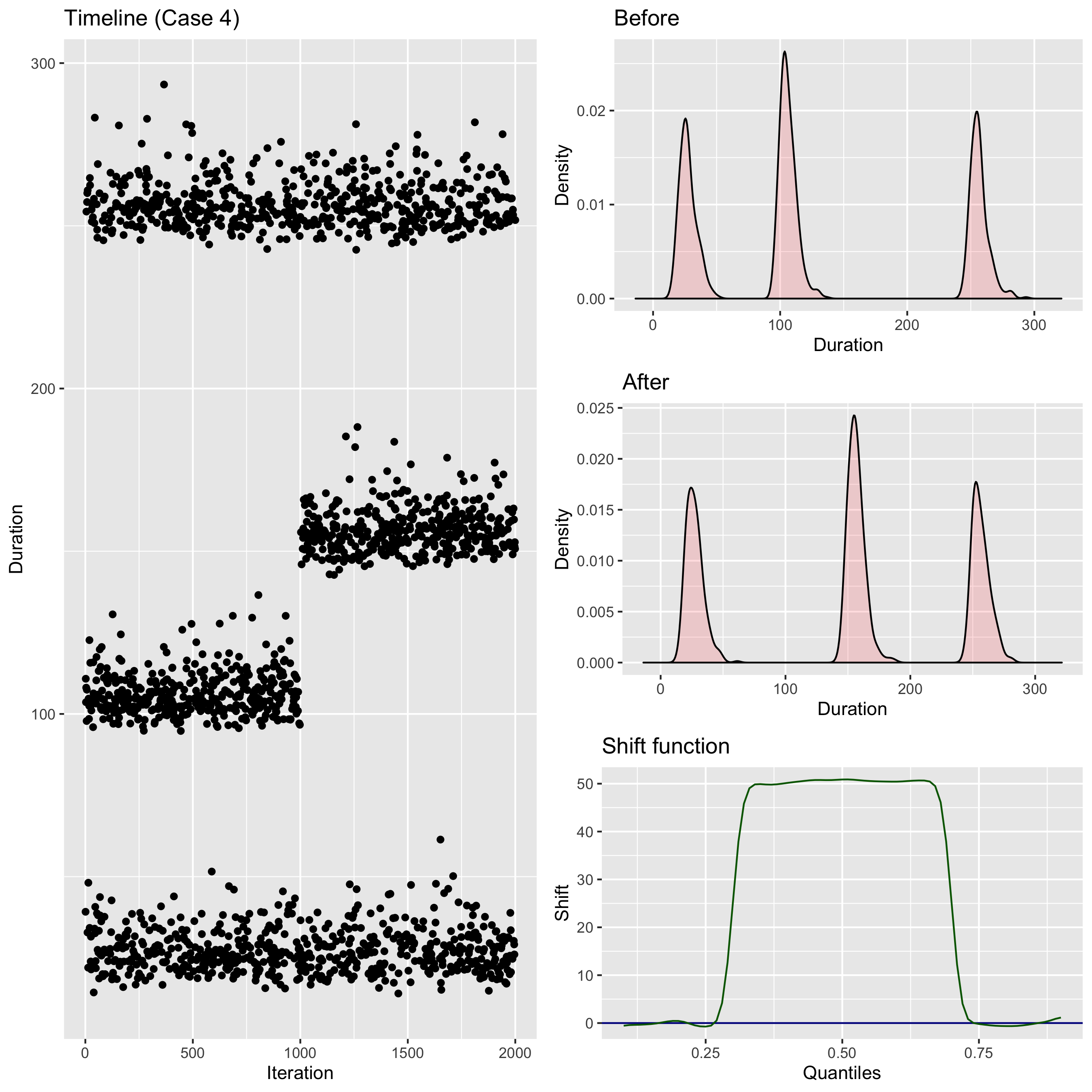
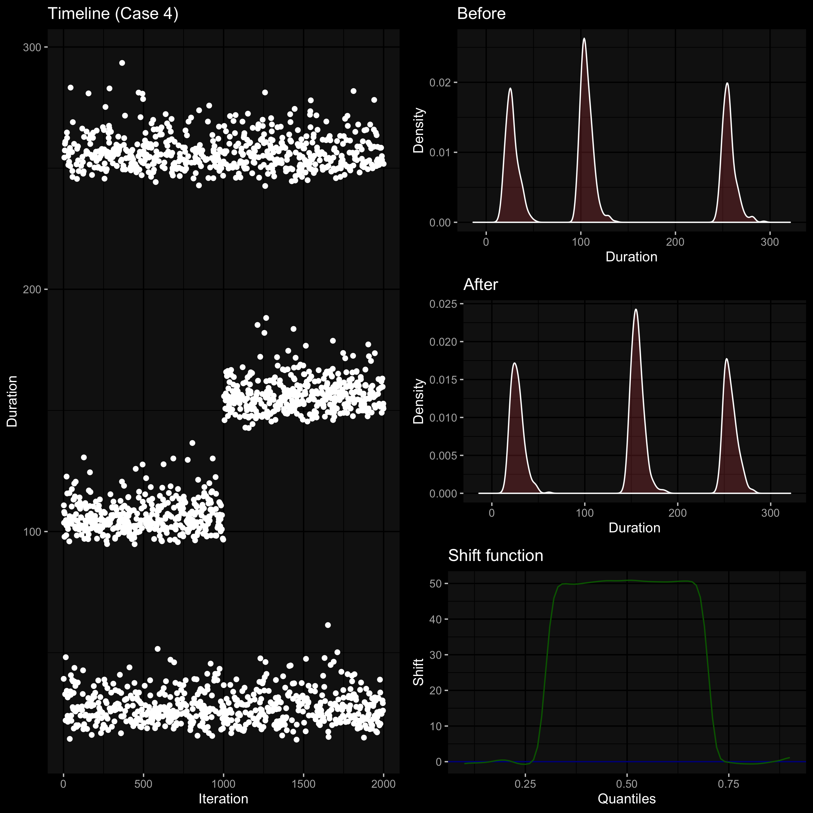
It shows the absolute shift for each quantile. The efficiency of the shift function can be improved with the help of the Harrell-Davis quantile estimator ( A new distribution-free quantile estimator
By Frank E Harrell, C E Davis · 1982 harrell1982).

Unfortunately, the raw shift function can’t be used as the effect size because it heavily depends on the distribution dispersion. Without it, we can’t say if the shift values are large or small. So, we need a way to normalize it.

MAD normalization

My favorite measure of the statistical dispersion is the median absolute deviation (MAD):

{MAD}_{X} = C \cdot median (| X_{i} - median (X) |), {MAD}_{Y} = C \cdot median (| Y_{i} - median (Y) |) .

For the normally distributed values, there is a well-known relationship between the standard deviation and the median absolute deviation:

s_{X} \approx 1.4826 \cdot median (| X_{i} - median (X) |) .

Thus, we can use $C = 1.4826$ (which is also known as the consistency constant) to make $MAD$ a consistent estimator for the standard deviation estimation.

By analogy with the pooled standard deviation, we can introduce the pooled median absolute deviation:

{PMAD}_{X Y} = \sqrt{\frac{(n_{X} - 1) {MAD}_{X}^{2} + (n_{Y} - 1) {MAD}_{Y}^{2}}{n_{X} + n_{Y} - 2}} .

As usual, we can use the Harrell-Davis quantile estimator to improve the efficiency of this metric.

A quantile-specific effect size

Now we are ready to write down the effect size for the given quantile $p$ . Let’s call it $γ_{p}$ (just because a lot of other good letters like d, Δ, g, Ψ, f, q, w, h are already occupied):

γ_{p} = \frac{Q_{p} (Y) - Q_{p} (X)}{{PMAD}_{X Y}}

where $Q_{p}$ is the $p^{th}$ quantile of the given sample.

For the normal distribution, the Cohen’s d equals to $γ_{0.5}$ :

d = \frac{\overset{―}{Y} - \overset{―}{X}}{s} \approx \frac{Q_{0.5} (Y) - Q_{0.5} (X)}{{PMAD}_{X Y}} = γ_{0.5} .

Condensation

It’s nice to have the effect size value for each specific quantile. However, it would be more convenient to have a single number (or a few numbers) that express the difference. Let’s introduce a set of the $γ_{p}$ values for an interval:

{\tilde{γ}}_{p} = {γ_{t} | t \in [p; 1 - p]} .

The shift function may be unstable around 0 and 1. Thus, it makes sense to drop these values and operate with the middle of the shift function. In practice, ${\tilde{γ}}_{0.2}$ or ${\tilde{γ}}_{0.3}$ work pretty well. For the given ${\tilde{γ}}_{p}$ , we can calculate the minimum and maximum values for this function across all quantiles:

min ({\tilde{γ}}_{p}) = min_{t \in [p; 1 - p]} γ_{t}, max ({\tilde{γ}}_{p}) = max_{t \in [p; 1 - p]} γ_{t} .

Finally, we can define a range of ${\tilde{γ}}_{p}$ :

range ({\tilde{γ}}_{p}) = [min ({\tilde{γ}}_{p}); max ({\tilde{γ}}_{p})] .

When the range is narrow, we can replace ${\tilde{γ}}_{p}$ by the minimum of the maximum value (or the average of these values). In practice, it will be a good way to describe the difference between two distributions using a single number.

When the range is wide, we can’t condensate ${\tilde{γ}}_{p}$ to a single number because the relationship between these distributions is too complex. In this case, it’s recommended to look at the plot of ${\tilde{γ}}_{p}$ (or just work with the range).

Reference implementation

If you use R, here is the function that you can use in your scripts:

library(Hmisc)

pooled <- function(x, y, FUN) {
  nx <- length(x)
  ny <- length(y)
  sqrt(((nx - 1) * FUN(x) ^ 2 + (ny - 1) * FUN(y) ^ 2) / (nx + ny - 2))
}
hdmedian <- function(x) as.numeric(hdquantile(x, 0.5))
hdmad <- function(x) 1.4826 * hdmedian(abs(x - hdmedian(x)))
phdmad <- function(x, y) pooled(x, y, hdmad)
gammaEffectSize <- function(x, y, prob)
  as.numeric((hdquantile(y, prob) - hdquantile(x, prob)) / phdmad(x, y))

If you use C#, you can take an implementation from the latest nightly version (0.3.0-nightly.33+) of Perfolizer (you need GammaEffectSize.CalcValue).

Conclusion

In this post, we built a new formula for the effect size:

γ_{p} = \frac{Q_{p} (Y) - Q_{p} (X)}{{PMAD}_{X Y}}, {\tilde{γ}}_{p} = {γ_{t} | t \in [p; 1 - p]} .

It provides the effect size for each quantile, but it can also be condensed to a range or a single number. It has the following advantages:

It’s robust
It’s applicable for nonparametric distributions.
It’s consistent with the Cohen’s d for normal distributions.
It’s not clamped, and it allows comparing large effect sizes for nonoverlapped distribution pairs.

I use this approach to compare distributions of software performance measurements (they are often right-skewed and heavily-tailed) in Rider. For my use cases, it works well and provides a good measure of the effect size. I hope it can be useful in many other applications. If you decide to try it, I will be happy to hear feedback about your experience.

References

[Cohen1988]
Cohen, Jacob. (1988). Statistical Power Analysis for the Behavioral Sciences. New York, NY: Routledge Academic
[Cliff1993]
Cliff, Norman. “Dominance statistics: Ordinal analyses to answer ordinal questions.” Psychological bulletin 114, no. 3 (1993): 494.
https://doi.org/10.1037/0033-2909.114.3.494
[Vargha2000]
Vargha A., and Delaney, H. D. “A critique and improvement of the CL common language effect size statistics of McGraw and Wong.” Journal of Educational and Behavioral Statistics, 25(2):101-132, 2000
https://doi.org/10.3102/10769986025002101
[Wilcox2019]
Wilcox, Rand. “A Robust Nonparametric Measure of Effect Size Based on an Analog of Cohen’s d, Plus Inferences About the Median of the Typical Difference.” Journal of Modern Applied Statistical Methods 17, no. 2 (2019): 1.
[Doksum1974]
Doksum, Kjell. “Empirical probability plots and statistical inference for nonlinear models in the two-sample case.” The annals of statistics (1974): 267-277.
https://doi.org/10.1214/aos/1176342662
[Doksum1976]
Doksum, Kjell A., and Gerald L. Sievers. “Plotting with confidence: Graphical comparisons of two populations.” Biometrika, 63, no. 3 (1976): 421-434.
https://doi.org/10.2307/2335720
[Harrell1982]
Harrell, F.E. and Davis, C.E., 1982. “A new distribution-free quantile estimator.” Biometrika, 69(3), pp.635-640.
https://pdfs.semanticscholar.org/1a48/9bb74293753023c5bb6bff8e41e8fe68060f.pdf