Normality is a myth

October 9, 2019 Mathematics Statistics Normality Central Limit Theorem

In many statistical papers, you can find the following phrase: “assuming that we have a normal distribution.” Probably, you saw plots of the normal distribution density function in some statistics textbooks, it looks like this:

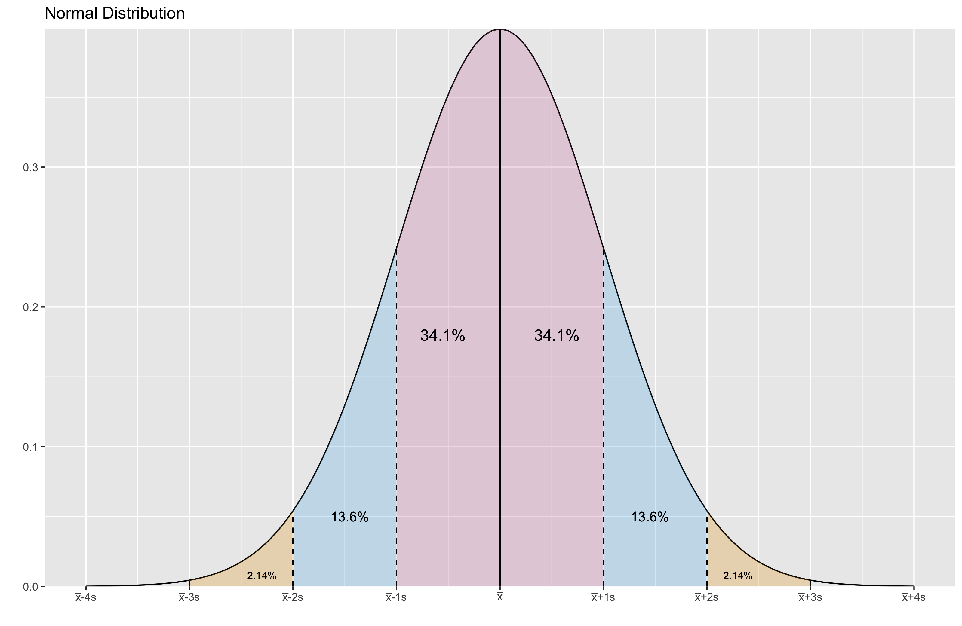
The normal distribution is a pretty user-friendly mental model when we are trying to interpret the statistical metrics like mean and standard deviation. However, it may also be an insidious and misleading model when your distribution is not normal. There is a great sentence in the “Testing for normality” paper by R.C. Geary, 1947 (the quote was found here):

Normality is a myth; there never was, and never will be, a normal distribution.

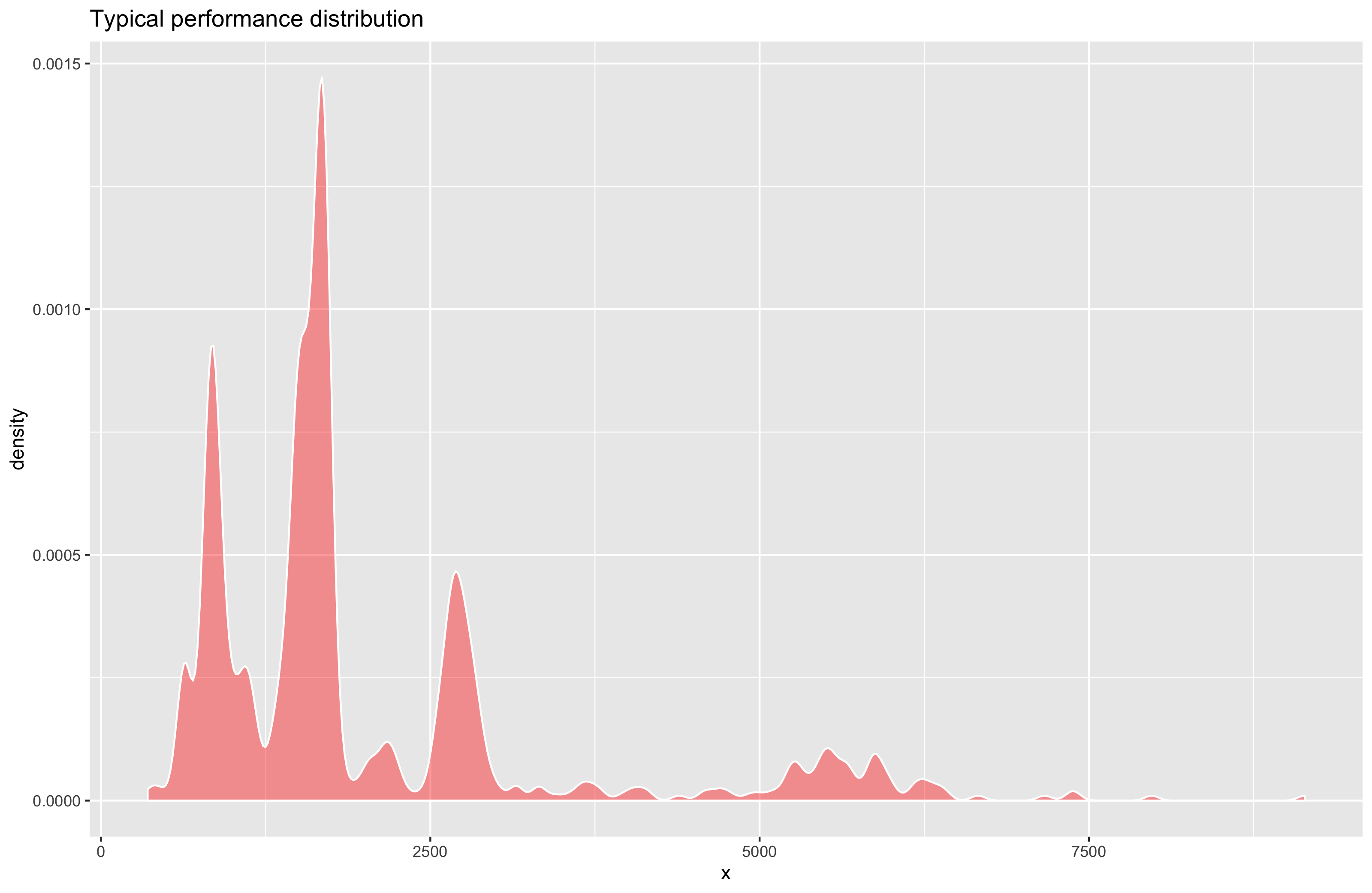
I 100% agree with this statement. At least, if you are working with performance distributions (that are based on the multiple iterations of your benchmarks that measure the performance metrics of your applications), you should forget about normality. That’s how a typical performance distribution looks like (I built the below picture based on a real benchmark that measures the load time of assemblies when we open the Orchard solution in Rider on Linux):

Of course, some of the performance distributions look similar to the normal distribution. And you can apply statistical approaches that assume normality to such distributions. And these approaches may provide correct results in many cases. If you are working with a single benchmark and manually check the results, you will be probably lucky enough and get correct results which will strengthen your faith to the fact that it’s OK to use such approaches all the time. However, if you are working with thousands of performance tests and you are trying to use such approaches automatically, you will probably get wrong results for some of these tests all the time.

The worst thing about the real performance distributions (that are often right-skewed and multimodal) is that it makes all of the statistical metrics (like the mean) misleading. Let’s look at an example of BenchmarkDotNet summary table:

| Method |     Mean |    Error |   StdDev |   Median |
|------- |---------:|---------:|---------:|---------:|
|      A | 136.2 ms | 19.30 ms | 56.92 ms | 107.0 ms |
|      B | 133.7 ms |  4.14 ms | 12.20 ms | 130.2 ms |

From my observations, when the Mean value is presented, people usually read only the Mean column and ignore other columns. After that, they make conclusions only based on the Mean values and the normal distribution mental model. Thus, they may think that B always works a little bit faster than A in the above table. Now let’s look at the “Expectation vs. Reality” picture for the A and B density plots:

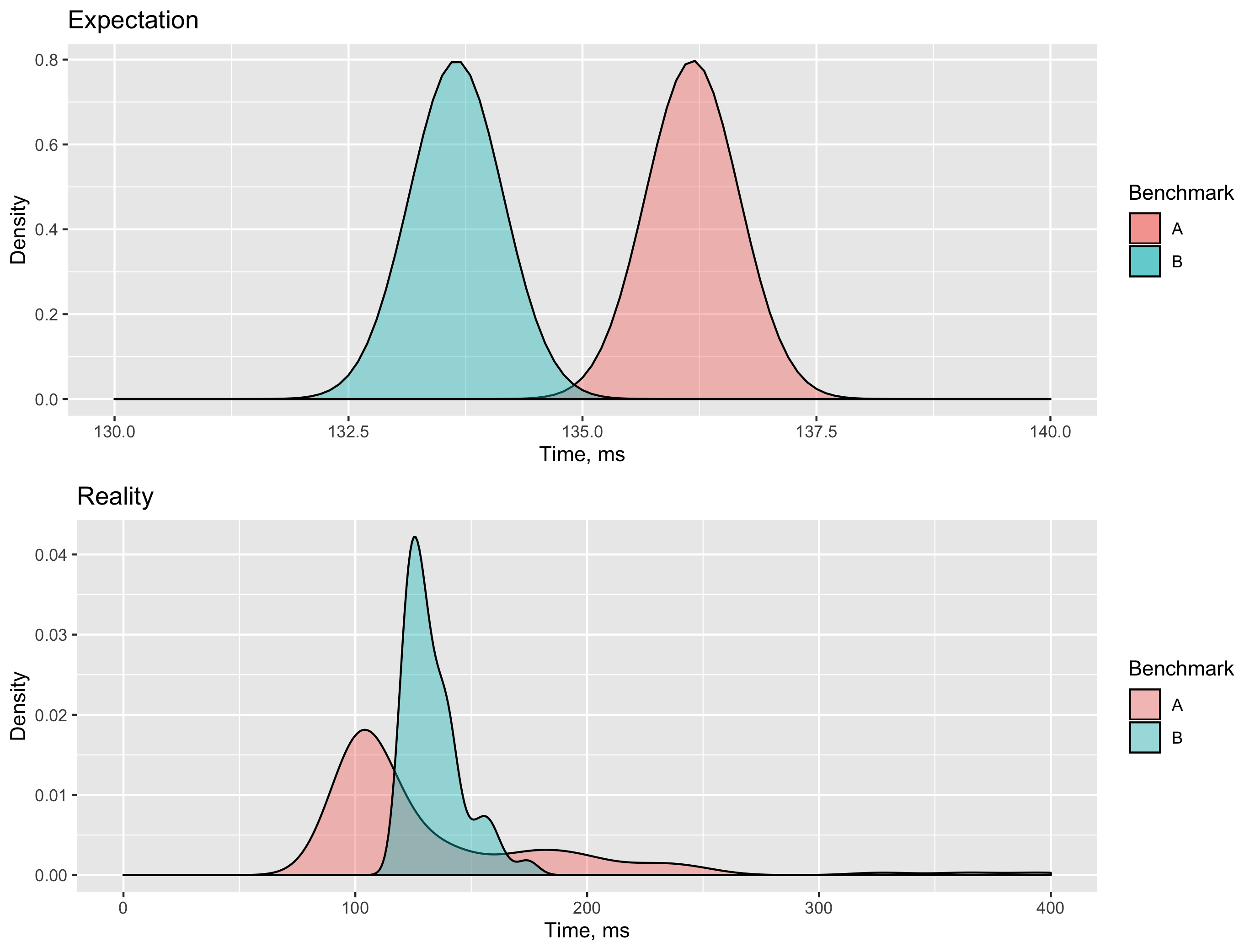
As you can see, both distributions are heavy-tailed right-skewed distributions. A has very huge outliers (that spoiled the mean value), but most of the B quantiles are larger than the corresponding A quantiles. BenchmarkDotNet automatically added the Median column to highlight this fact (the median value for B is much larger than the median value for A). Unfortunately, most of the people ignore such kind of additional information and continue to imagine a normal distribution based on the mean value.

There is one more thing in perception of statistics. When I tell people about complex multimodal heavy-tailed right-skewed distributions, they usually reply that we have the Central Limit Theorem. For some reason, people think that it will magically stabilize the mean value and rescue us from multimodal distributions if we collect “enough” measurements. Here is the definition of this theorem from Statistics For Dummies:

The Central Limit Theorem (CLT for short) basically says that for non-normal data, the distribution of the sample means has an approximate normal distribution, no matter what the distribution of the original data looks like, as long as the sample size is large enough (usually at least 30) and all samples have the same size.

So, if we take many samples (sets of measurements), calculate the mean value for each sample, and build a distribution from these mean values, it should be normal. If you are not sure that you understand the Central Limit Theorem, I you can watch this video that explains it with Bunnies & Dragons (the original was found here):

Let’s check how it works in practice. I wrote a simple R script that emulates taking measurements from a “strange” distribution with high outliers:

library(ggplot2)

n <- 30 # Number of values in each sample
m <- 30 # Number of samples
k <- 16 # Number of CLT distributions

set.seed(159)
# Generate a single random value from a "strange" distribution
gen.value <- function()
  sample(1:10, 1) +                               # Offset
  rbeta(1, 1, 10) * sample(1:10, 1) +             # Right-skewed distribution
  sample(c(rep(0, 50), 1:10)) * rnorm(1, 200, 10) # Outliers
# Generate a sample mean
gen.mean <- function() mean(sapply(1:n, function(x) gen.value()))

df <- data.frame()
for (i in 1:k) {
  df <- rbind(df, data.frame(
    Experiment = rep(i, m),
    Time = sapply(1:m, function(j) gen.mean()))
  )
}
p <- ggplot(df, aes(x = Time, group = Experiment)) +
  geom_density(fill = "red", alpha = 0.4, bw = "SJ") +
  facet_wrap(~Experiment) +
  ylab("Density")

In this script, gen.value returns a random value from our “strange” distribution, gen.mean generates a sample with 30 measurements (because 30 is a magic number) and returns the mean value of this sample. Next, we perform 16 experiments. In each experiment, we draw a distribution density function based on 30 mean values that we generated. Here is the result:

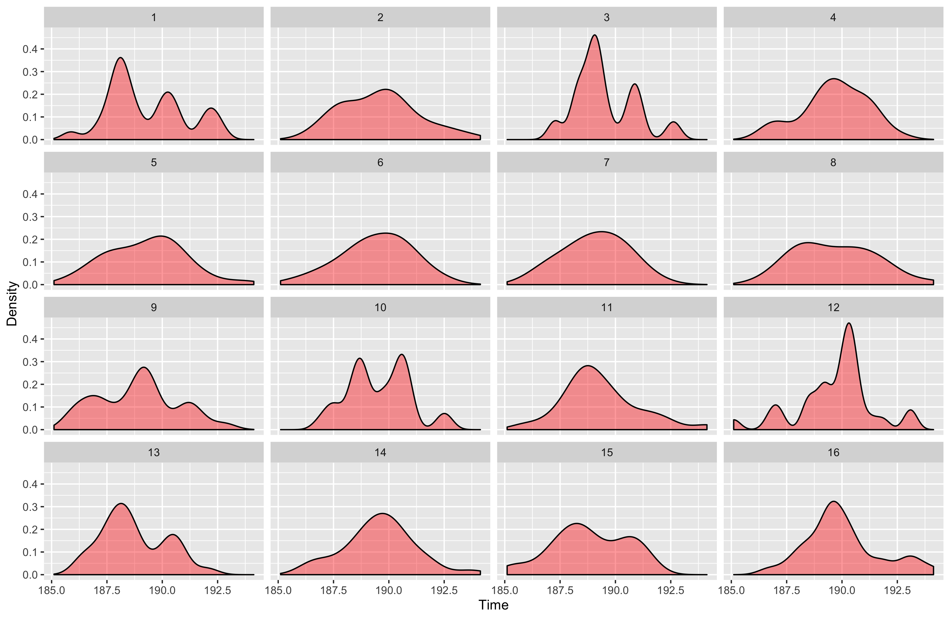
As you can see, many of the generated distribution are not looking as normal. What’s wrong? Maybe the Central Limit Theorem doesn’t work? Don’t worry, there are no problems with the theorem. We just didn’t take enough measurements. If we increase the sample sizes (n and m parameters in the above R script), the plots will be “fixed”: the observed density plots will become “more normal.”

Now let’s think about the sample sizes. In each experiment, we draw a density function based on 900 measurements (we have 30 mean values; each value was calculated based on a sample with 30 measurements). The script works pretty fast because it generates “fake” data. In real life, we typically spend at least 1 second per measurement. If we want to build such a plot based on the real data, we will spend 900 seconds (or 15 minutes) per an experiment. Some of the real benchmarks may take more than 1 minute per measurement which means that we should spend 15 hours for the whole experiment. In theory, if we spend a lot of hours on the measurements, we will most likely get a plot which will be similar to the normal distribution. In practice, we will not spend so much time per each benchmark (especially, if we have hundreds or thousands of them).

At the conclusion, I want to highlight some important facts about the Central Limit Theorem that people usually don’t understand (based on the “The Central Limit Theorem” section from my book):

If we do many iterations, the original distribution will not become normal, and we can’t interpret the mean, the variance, the skewness, and the kurtosis as in the case of normal distribution.
The range of the mean values across all samples is not always narrow, we still can have a huge difference between the mean values in different samples. The normal distribution based on the mean values has its own standard deviation which depends on the sample size and can be expressed via the standard error.
The central limit theorem doesn’t work correctly when the sample sizes are small. For example, if you make a single measurement in each sample, the distribution based on the mean values will have the same shape as the original distribution.
If we take a small number of samples ($n < 100$), we will probably not see a normal distribution on the density plot for mean values.

If we are speaking about the original performance distributions, we can forget about normality at all. The assumption of normality can work fine in some special cases, but it will let you down in the long run. Remember the R.C. Geary’s words: “Normality is a myth; there never was, and never will be, a normal distribution.”