Partial binning compression of performance series
Let’s start with a problem from real life. Imagine we have thousands of application components that should be initialized. We care about the total initialization time of the whole application, so we want to automatically track the slowest components using a continuous integration (CI) system. The easiest way to do it is to measure the initialization time of each component in each CI build and save all the measurements to a database. Unfortunately, if the total number of components is huge, the overall artifact size may be quite extensive. Thus, this approach may introduce an unwanted negative impact on the database size and data processing time.
However, we don’t actually need all the measurements. We want to track only the slowest components. Typically, it’s possible to introduce a reasonable threshold that defines such components. For example, we can say that all components that are initialized in less than 1ms are “fast enough,” so there is no need to know the exact initialization time for them. Since these time values are insignificant, we can just omit all the measurements below the given thresholds. This allows to significantly reduce the data traffic without losing any important information.
The suggested trick can be named partial binning compression. Indeed, we introduce a single bin (perform binning) and omit all the values inside this bin (perform compression). On the other hand, we don’t build an honest histogram since we keep all the raw values outside the given bin (the binning is partial).
Let’s discuss a few aspects of using partial binning compression.
Data reconstruction
The data reconstruction process is pretty straightforward. Let’s say we want to build a series of initialization durations for the given component. For each build with existing measurement for this component, we just use this measurement. For each build without any records for this component, we use a special “binned” value that specifies that the original value is below the given threshold.
Here is an example of such a performance series with 1ms threshold:
[0;1]ms, [0;1]ms, [0;1]ms, [0;1]ms, [0;1]ms, 15ms, 16ms, 16ms, 15ms, 17ms
We can see that the first five measurements are below 1ms, the last five measurements are about 15-17ms. Thus, we can assume that there is a performance degradation in the middle of this series.
Data visualization
The typical density estimation for continuos data is a smooth density plot (e.g., using KDE or QRDE). The typical density estimation for binned data is a histogram. Since we have partially binned data, we can introduce a hybrid of a smooth density plot and a histogram:
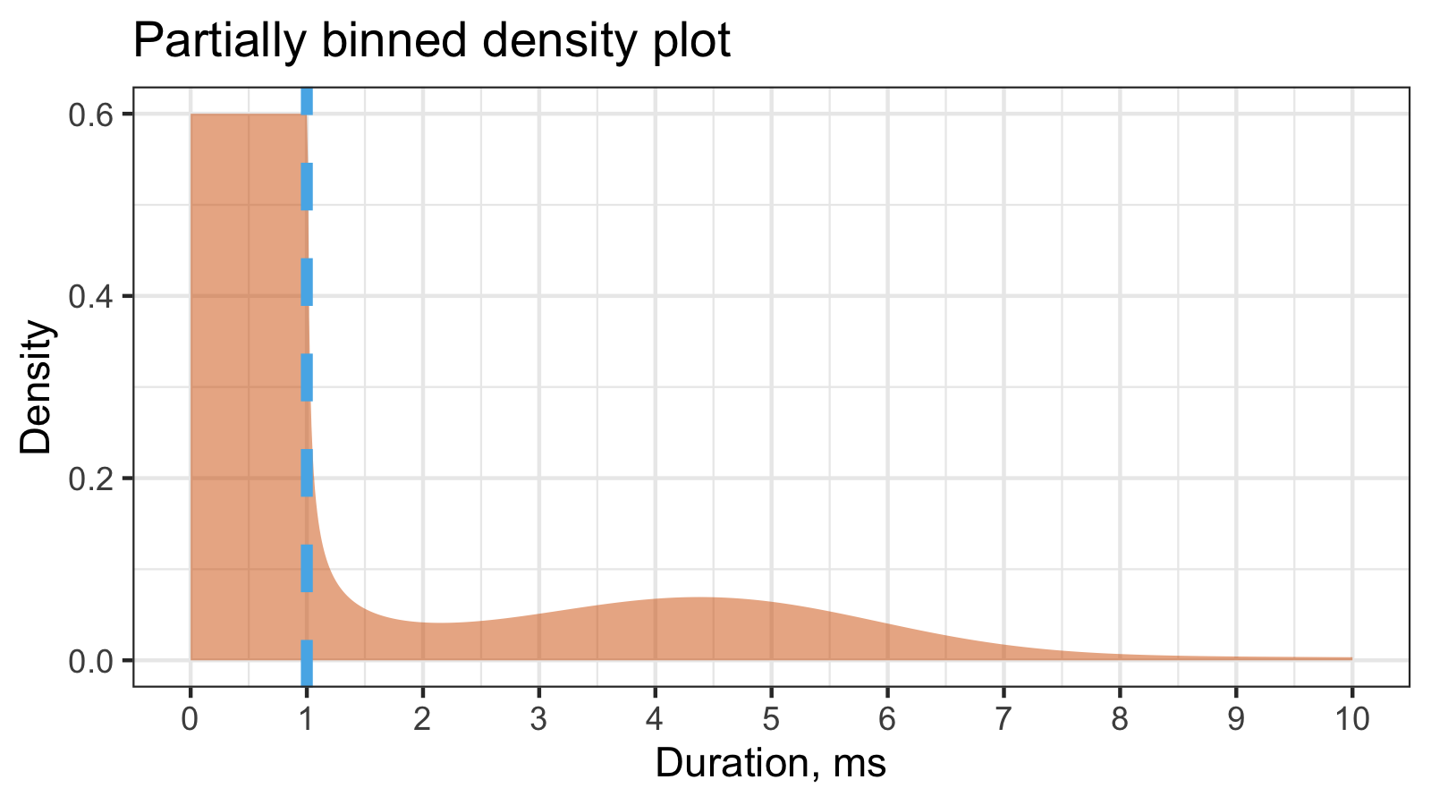

In this example, we have 60% of binned measurements inside the [0;1]ms interval and
40% of continuous measurements above the 1ms threshold.
Data analysis
In fact, the suggested partial binning introduces artificial bimodality. The first mode is the single bin, the second mode is all continuous values outside the bin. If we want to compare two samples, the first thing we have to do is to compare the proportion between two modes in each sample. For example, let’s consider two following samples with 1000 elements in each sample:
| [0;1]ms | >1ms | |
|---|---|---|
| Sample 1 | 312 | 688 |
| Sample 2 | 647 | 353 |
There are 312 binned elements in the first sample and 647 binned elements in the second sample. Thus, we can assume that the second sample is probably faster.
The second thing we can do is to compare non-binned elements of both samples. For example, let’s consider the following two samples:
Sample1: [0;1]ms, [0;1]ms, [0;1]ms, [0;1]ms, [0;1]ms,  15ms,  16ms,  16ms,  15ms,  17ms
Sample2: [0;1]ms, [0;1]ms, [0;1]ms, [0;1]ms, [0;1]ms, 218ms, 225ms, 219ms, 224ms, 221ms
The proportion between two modes is the same for both samples, but the second sample has higher non-binned values. Thus, we can assume that the first sample is probably faster.
Since we work with non-parametric distributions, we are not always able to unequivocally compare samples. For example, the portion of the binned values can be better in the first sample, but the magnitude of the non-binned values can be better in the second sample. In such cases, we can compare samples using the shift and ration functions or the effect size function. All these techniques can be easily generalized for the partially binned samples.
Conclusion
The suggested partial binning compression allows reducing the amount of kept data without losing important information. Meanwhile, we are still able to produce basic operations on obtained samples like visualization and analysis.