MP² quantile estimator: estimating the moving median without storing values

In one of the previous posts, I described the P² quantile estimator. It allows estimating quantiles on a stream of numbers without storing them. Such sequential (streaming/online) quantile estimators are useful in software telemetry because they help to evaluate the median and other distribution quantiles without a noticeable memory footprint.

After the publication, I got a lot of questions about moving sequential quantile estimators. Such estimators return quantile values not for the whole stream of numbers, but only for the recent values. So, I wrote another post about a quantile estimator based on a partitioning heaps (inspired by the Hardle-Steiger method). This algorithm gives you the exact value of any order statistics for the last $L$ numbers ($L$ is known as the window size). However, it requires $O(L)$ memory, and it takes $O(log(L))$ time to process each element. This may be acceptable in some cases. Unfortunately, it doesn’t allow implementing low-overhead telemetry in the case of large $L$.

In this post, I’m going to present a moving modification of the P² quantile estimator. Let’s call it MP² (moving P²). It requires $O(1)$ memory, it takes $O(1)$ to process each element, and it supports windows of any size. Of course, we have a trade-off with the estimation accuracy: it returns a quantile approximation instead of the exact order statistics. However, in most cases, the MP² estimations are pretty accurate from the practical point of view.

Let’s discuss MP² in detail!

The idea

The approach behind the P² quantile estimator is elegant, so I recommend reading it first. However, it’s not required: we are going to use it as a black box. We are going to consider an approach that can be applied for “movification” of any sequential quantile estimator.

Let me show the main idea on a simple example with window size $L = 100$. Imagine that we processed the first 230 elements of our stream $x$:

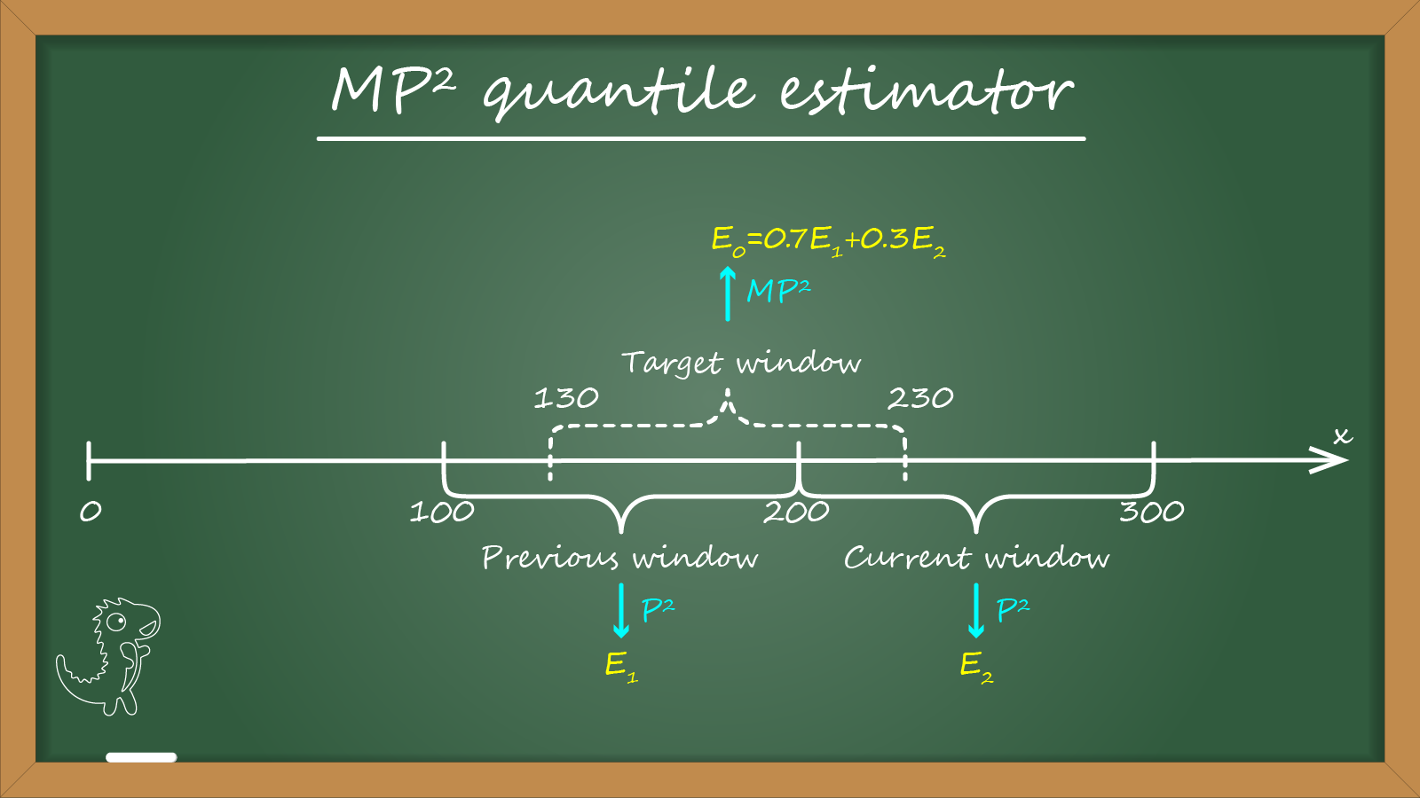
We want to estimate the quantile value for the last $100$ elements. It gives us the following range (assuming one-based indexing):

• $x_{131}..x_{230}$ (the “target” window).

Let’s build a quantile estimator that gives an estimation $E_0$ for the “target” window. Instead of direct quantile estimating inside this window, we are going to work with two non-overlapped fixed-offset windows:

• $x_{101}..x_{200}$ (the “previous” window).
• $x_{201}..x_{300}$ (the “current” window).

We assume that the quantile estimation for the previous window is known. For the current window, we maintain an independent P² quantile estimator that accumulate the observed values. Let’s introduce the following notation:

• $E_1$: the known quantile estimation for the previous window.
• $E_2$: the current quantile estimation for the current window based on the P² quantile estimator.
• $k$: the number of processed elements inside the current window.

Now we can approximate the quantile value for the target window using the following equation:

The target estimation $E_0$ is a weighted sum of two existing estimates $E_1$ and $E_2$:

• The weight of $E_1$ is $(L-k)/L$ because the previous window covers $L-k$ elements of the target window.
• The weight of $E_2$ is $k/L$ because the current window covers $k$ elements of the target window.

For the above example, $k=30$ (because we have processed only $x_{201}..x_{230}$ from the current window), $L=100$. Thus, $E_0 = ((100-30) E_1 + 30E_2)/100 = 0.7E_1 + 0.3E_2$.

I hope you got the main idea. Now it’s time to formalize the algorithm. Let’s say, we process the $n^{\textrm{th}}$ element. Depending on $n$, we should do the following (assuming one-based indexing):

• For $1 \leq n \leq L$:
  • Process $x_n$ by the internal P² quantile estimator
  • Use $E_0 = E_2$
• For $n \geq L,\; n \bmod L \neq 1$:
  • Process $x_n$ by the internal P² quantile estimator
  • Assign $k = \big( (n + L - 1) \bmod L \big) + 1$
  • Use $E_0 = \big( (L-k) \cdot E_1 + k \cdot E_2 \big) / L$
• For $n \geq L,\; n \bmod L = 1$:
  • Assign $E_1 = E_2$
  • Restore the internal P² quantile estimator to the initial state
  • Process $x_n$ by the internal P² quantile estimator
  • Use $E_0 = \big( (L-k) \cdot E_1 + k \cdot E_2 \big) / L$

Numerical simulations

One of my favorite data sets for testing moving median estimators is a noisy sine wave pattern with high outliers.¹ Let’s try to use the MP² quantile estimator with such a data set (the source code is here):

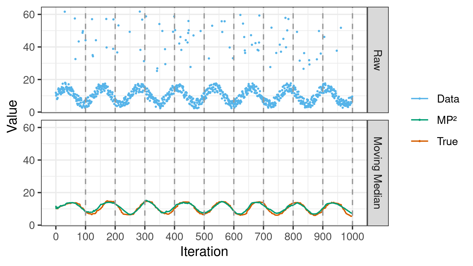
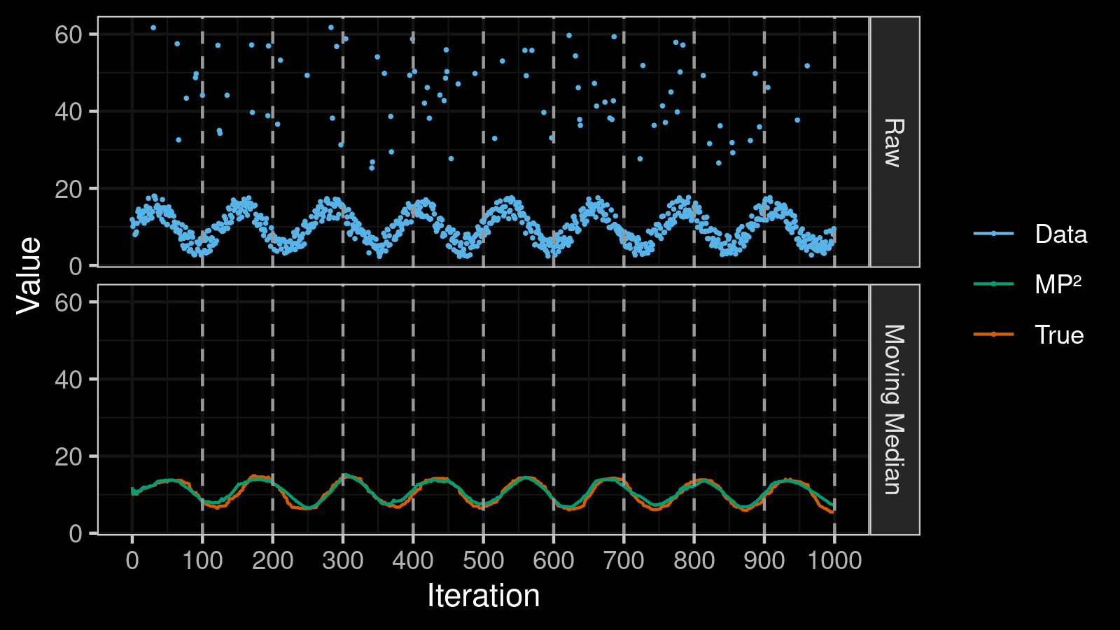
Here we can do the following observations:

• The moving median correctly shows the primary sine wave trend; it’s not affected by the outliers.
• The estimations of the MP² quantile estimator (the green “MP²” line in the bottom chart) are pretty close to the true values of the moving median (the orange “True” line in the bottom chart).
• On the borders between considered fixed-offset windows, the MP² estimations and the true values are almost synced. These points correspond to the native accuracy of the P² quantile estimator. We have some deviations between these points, but they are usually minor.

Currently, I don’t have the accuracy estimations for the suggested estimator. However, it shows decent results in multiple numerical simulations on synthetic and real data sets.

Reference implementation

If you use C#, you can take an implementation from the latest nightly version (0.3.0-nightly.82+) of Perfolizer (you need MovingP2QuantileEstimator).

Below you can find a standalone copy-pastable implementation of the suggested estimator.

public class P2QuantileEstimator
{
    private readonly double p;
    private readonly int[] n = new int[5];
    private readonly double[] ns = new double[5];
    private readonly double[] dns = new double[5];
    private readonly double[] q = new double[5];
    private int count;

    public P2QuantileEstimator(double probability)
    {
        p = probability;
    }

    public void Add(double value)
    {
        if (count < 5)
        {
            q[count++] = value;
            if (count == 5)
            {
                Array.Sort(q);

                for (int i = 0; i < 5; i++)
                    n[i] = i;

                ns[0] = 0;
                ns[1] = 2 * p;
                ns[2] = 4 * p;
                ns[3] = 2 + 2 * p;
                ns[4] = 4;

                dns[0] = 0;
                dns[1] = p / 2;
                dns[2] = p;
                dns[3] = (1 + p) / 2;
                dns[4] = 1;
            }

            return;
        }

        int k;
        if (value < q[0])
        {
            q[0] = value;
            k = 0;
        }
        else if (value < q[1])
            k = 0;
        else if (value < q[2])
            k = 1;
        else if (value < q[3])
            k = 2;
        else if (value < q[4])
            k = 3;
        else
        {
            q[4] = value;
            k = 3;
        }

        for (int i = k + 1; i < 5; i++)
            n[i]++;
        for (int i = 0; i < 5; i++)
            ns[i] += dns[i];

        for (int i = 1; i <= 3; i++)
        {
            double d = ns[i] - n[i];
            if (d >= 1 && n[i + 1] - n[i] > 1 || d <= -1 && n[i - 1] - n[i] < -1)
            {
                int dInt = Math.Sign(d);
                double qs = Parabolic(i, dInt);
                if (q[i - 1] < qs && qs < q[i + 1])
                    q[i] = qs;
                else
                    q[i] = Linear(i, dInt);
                n[i] += dInt;
            }
        }

        count++;
    }

    private double Parabolic(int i, double d)
    {
        return q[i] + d / (n[i + 1] - n[i - 1]) * (
            (n[i] - n[i - 1] + d) * (q[i + 1] - q[i]) / (n[i + 1] - n[i]) +
            (n[i + 1] - n[i] - d) * (q[i] - q[i - 1]) / (n[i] - n[i - 1])
        );
    }

    private double Linear(int i, int d)
    {
        return q[i] + d * (q[i + d] - q[i]) / (n[i + d] - n[i]);
    }

    public double GetQuantile()
    {
        if (count == 0)
            throw new IndexOutOfRangeException("There are no any values");
        if (count <= 5)
        {
            Array.Sort(q, 0, count);
            int index = (int) Math.Round((count - 1) * p);
            return q[index];
        }

        return q[2];
    }

    public void Clear()
    {
        count = 0;
    }
}

public class MovingP2QuantileEstimator
{
    private readonly P2QuantileEstimator estimator;
    private readonly int windowSize;
    private int n;
    private double previousWindowEstimation;

    public MovingP2QuantileEstimator(double probability, int windowSize)
    {
        this.windowSize = windowSize;
        estimator = new P2QuantileEstimator(probability);
    }

    public void Add(double value)
    {
        n++;
        if (n % windowSize == 0)
        {
            previousWindowEstimation = estimator.GetQuantile();
            estimator.Clear();
        }
        estimator.Add(value);
    }

    public double GetQuantile()
    {
        if (n == 0)
            throw new IndexOutOfRangeException("There are no values");
        if (n < windowSize)
            return estimator.GetQuantile();
        
        double estimation1 = previousWindowEstimation;
        double estimation2 = estimator.GetQuantile();
        double w2 = (n % windowSize + 1) * 1.0 / windowSize;
        double w1 = 1.0 - w2;
        return w1 * estimation1 + w2 * estimation2;
    }
}

Conclusion

Here are the main characteristics of the presented MP² quantile estimator:

• Memory: $O(1)$.
  It requires only three additional variables in comparison with the P² quantile estimator (the window size $L$, the number of processed elements $n$, the quantile estimation for the previous window $E_1$).
• Element processing complexity: $O(1)$.
  The algorithm involves a small number of simple arithmetic operations that don’t depend on the window size.
• Quantile estimation complexity: $O(1)$.
  Since we always have ready $E_1$ and $E_2$ estimations, we have to just evaluate a simple formula.

The accuracy is not perfect, but it should be acceptable in most real-life scenarios.

The MP² quantile estimator may be useful in software performance telemetry. It provides a fast approach to estimate the median (and other quantiles) of collected performance measurements without noticeable memory overhead.