Quantile absolute deviation of the Exponential distribution

In this post, we derive the exact equation for the quantile absolute deviation around the median of the Exponential distribution.

Preparation

We consider the quantile absolute deviation around the median defined as follows:

$$ \newcommand{\E}{\mathbb{E}} \newcommand{\PR}{\mathbb{P}} \newcommand{\Q}{\operatorname{Q}} \newcommand{\QAD}{\operatorname{QAD}} \newcommand{\median}{\operatorname{median}} \newcommand{\Exp}{\operatorname{Exp}} \QAD(X, p) = \Q(|X - \median(X)|, p), $$

where $\Q$ is a quantile estimator.

We are looking for the asymptotic value of $\QAD(X, p)$. For simplification, we denote it by $v_p$:

$$ v_p = \lim_{n \to \infty} \E[\Q(|X-M|, p)], $$

where $M$ is the true median of the distribution.

By the definition of quantiles, this can be rewritten as:

$$ \PR(|X_1 - M| < v_p) = p, $$

which is the same as

$$ \PR(-v_p < X_1 - M < v_p) = p. $$

Hence,

$$ \PR(M - v_p < X_1 < M + v_p) = p. $$

If $F$ is the CDF of the considered distribution, the above equality can be rewritten as

$$ F(M + v_p) - F(M - v_p) = p. \tag{1} $$

Exponential distribution

We consider the standard exponential distribution $\Exp(1)$ given by the CDF $F(x)=1 - e^{-x}$ with the median value $M=\ln 2$. Since $F$ is defined only for $x > x_{\min} = 0$, we have to consider two cases: $M - v_p \leq 0$ and $M - v_p > 0$. The critical value $v_p^*$ is defined by $v_p^* = M - x_{\min} = M = \ln 2$. Now it is easy to get the value of $p^*$ using (1):

$$ p^* = F(2M - x_{\min}) = F(2M) = 1 - e^{-2\ln 2} = 1 - 0.25 = 0.75. $$

Let us consider the first case when $p \leq p^* = 0.75$. From (1), we have:

$$ (1 - e^{-\ln 2 - v_p}) - (1 + e^{-\ln 2 + v_p}) = p, $$

which is the same as

$$ e^{v_p} - e^{-v_p} = 2p. $$

By multiplying both sides of the equation by $e^{v_p}$, we get:

$$ (e^{v_p})^2 - 2p \cdot (e^{v_p}) - 1 = 0. $$

This is a quadratic equation for $e^{v_p}$ with coefficients $a=1$, $b=-2p$, $c=-1$. The discriminant is given by $D = b^2 - 4ac = 4p^2 + 4$. The solution of the quadratic equation is

$$ e^{v_p} = \frac{-b \pm \sqrt{D}}{2a} = \frac{2p \pm \sqrt{4p^2 + 4}}{2} = p \pm \sqrt{p^2+1}. $$

Since $e^{v_p}$ is always positive, only the plus is applicable for $\pm$. Taking the natural logarithm from both parts, we get the result:

$$ v_p = \ln(p + \sqrt{p^2+1}). $$

Now let us consider the second case when $p > p^* = 0.75$. Equation (1) has the following form:

$$ (1 - e^{-\ln 2 - v_p}) = p, $$

which is the same as

$$ e^{-\ln 2 - v_p} = 1 - p. $$

Taking the natural logarithm from both parts, we can easily express $v_p$:

$$ v_p = -\ln 2 - \ln (1 - p). $$

Thus, if $X \sim \Exp(1)$,

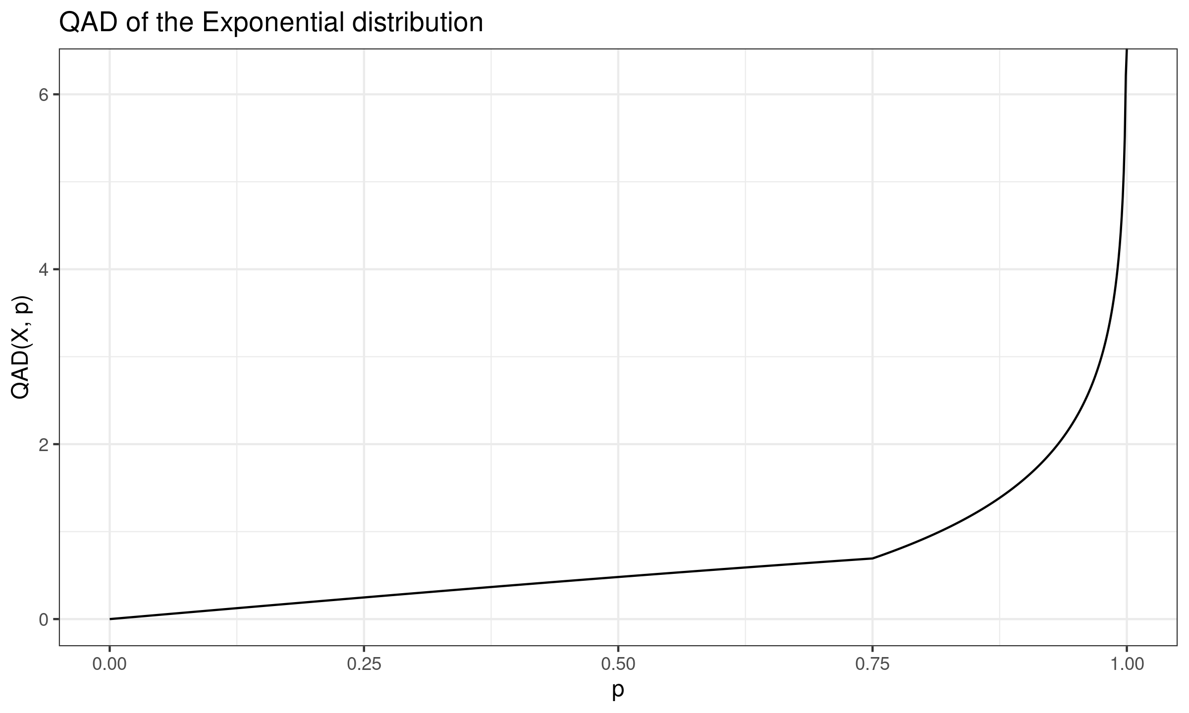
$$ \lim_{n \to \infty} \E[\QAD(X, p)] = \begin{cases} \ln(p + \sqrt{p^2+1}), & \textrm{if}\; p \leq 0.75,\\ -\ln 2 - \ln (1 - p), & \textrm{if}\; p > 0.75. \end{cases} $$

Here is the corresponding plot: