Quantile absolute deviation: estimating statistical dispersion around quantiles
The below text contains an intermediate snapshot of the research and is preserved for historical purposes.
There are many different metrics for statistical dispersion. The most famous one is the standard deviation. The standard deviation is the most popular way to describe the spread around the mean when you work with normally distributed data. However, if you work with non-normal distributions, this metric may be misleading.
In the world of non-parametric distributions, the most common measure of central tendency is the median. For the median, you can describe dispersion using the median absolute deviation around the median (MAD). It works great if the median is the only summary statistic that you care about. However, if you work with multimodal distributions (they can be detected using the lowland multimodality detector), you may be interested in other quantiles as well. So, it makes sense to learn how to describe dispersion around the given quantile. Which metric should we choose?
Recently, I came up with a great solution to this problem. We can generalize the median absolute deviation into the quantile absolute deviation (QAD) around the given quantile based on the Harrell-Davis quantile estimator. I will show how to calculate it, how to interpret it, and how to get insights about distribution properties from images like this one:
Median absolute deviation around the median
Let’s start with the classic definition for the median absolute deviation around the median:
$$ \mathcal{MAD}(x) = C \cdot \textrm{median}(|x_i - \textrm{median}(x)|). $$Here $C$ is a scale factor. Typically, $C \approx 1.4826$ to use $\mathcal{MAD}$ a consistent estimator for the estimation of the standard deviation in the case of the normal distribution. In the scope of this post, there is no need to be consistent with other dispersion metrics, so you can assume that $C = 1$.
When people use the $\mathcal{MAD}$, they usually forget to pay attention to the quantile estimator that
is used to calculate the median.
Meanwhile, the quantile estimator heavily affects the efficiency of the final version.
For further discussion, let’s use the Harrell-Davis quantile estimator (
A new distribution-free quantile estimator
By Frank E Harrell, C E Davis
·
1982harrell1982)
because it’s one of the most smooth and efficient options.
One of the most important properties of the $\mathcal{MAD}$ you should know: the range $[\textrm{median}(x) - \mathcal{MAD}(x); \textrm{median}(x) + \mathcal{MAD}(x)]$ contains 50% of the distribution:
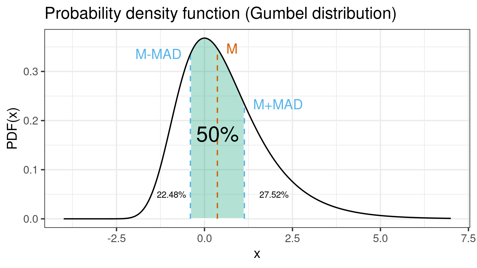
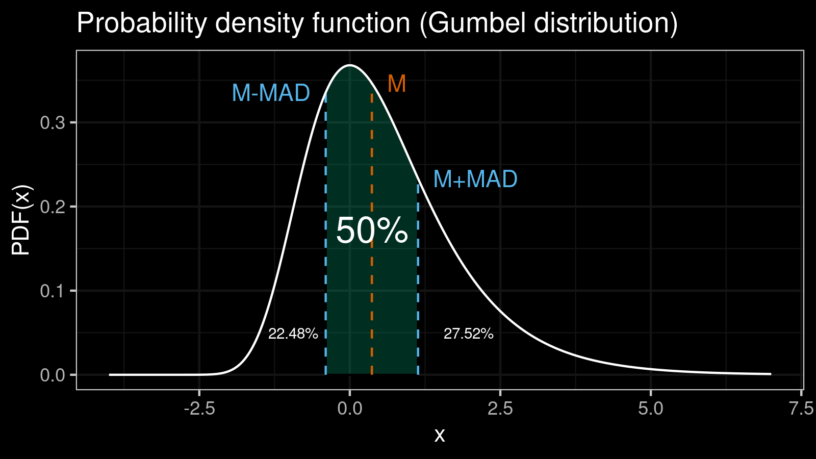
For better understanding, you can check out an example of how to calculate the exact value of the $\mathcal{MAD}$ for the Gumbel distribution.
Median absolute deviation around quantiles
The above formula looks great for the median, but what if we want to describe dispersion for a quantile? By analogy, we can build the median absolute deviation around the $p^{\textrm{th}}$ quantile:
$$ \mathcal{MAD}(x, p) = C \cdot \textrm{median}(|x_i - Q(x, p)|), $$where $Q(x; p)$ is the $p^{\textrm{th}}$ quantile of $x$.
It works similar way as the classic $\mathcal{MAD}$ around the median: the interval $[Q(x, p) - \mathcal{MAD}(x, p); Q(x, p) + \mathcal{MAD}(x, p)]$ contains exactly 50% of the distribution.
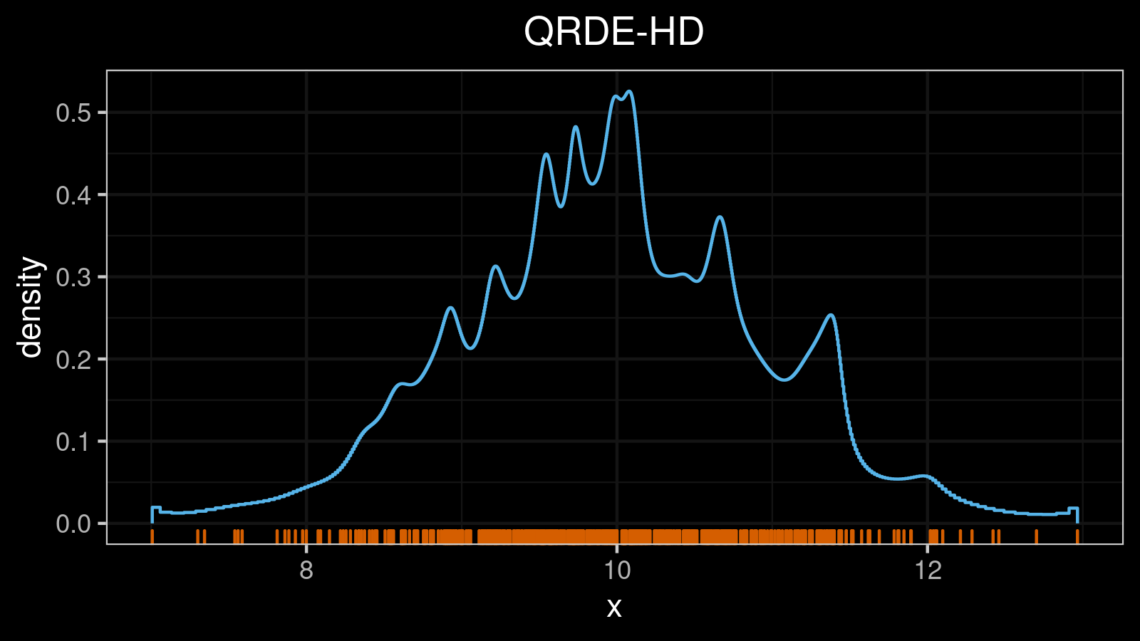
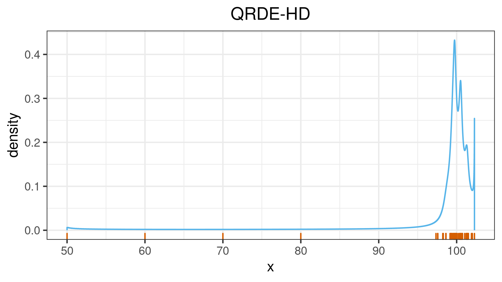
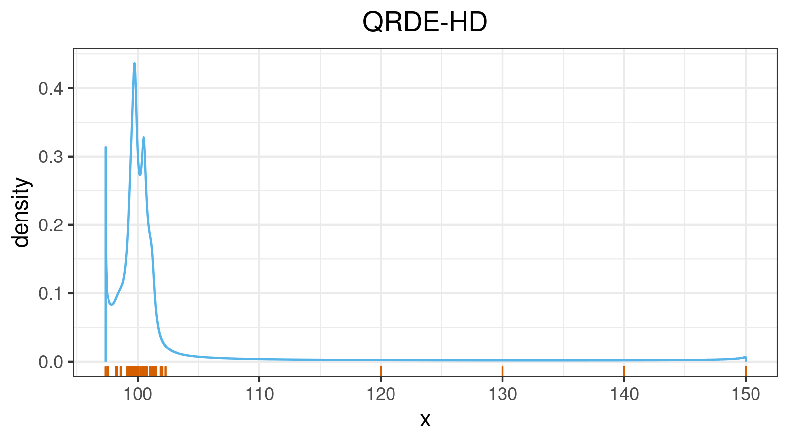
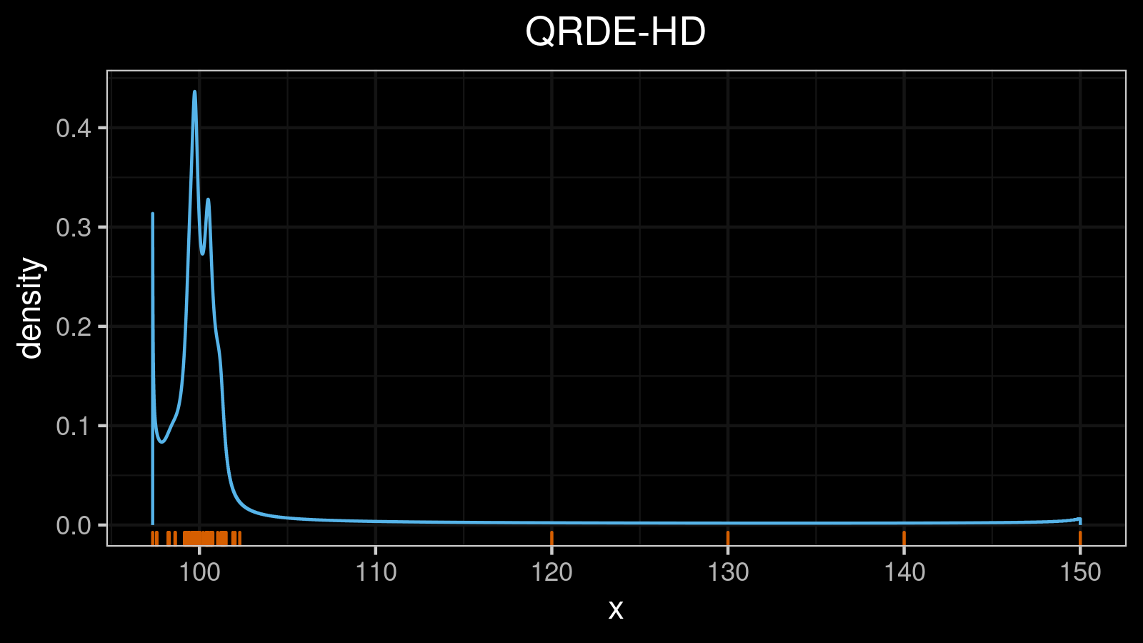
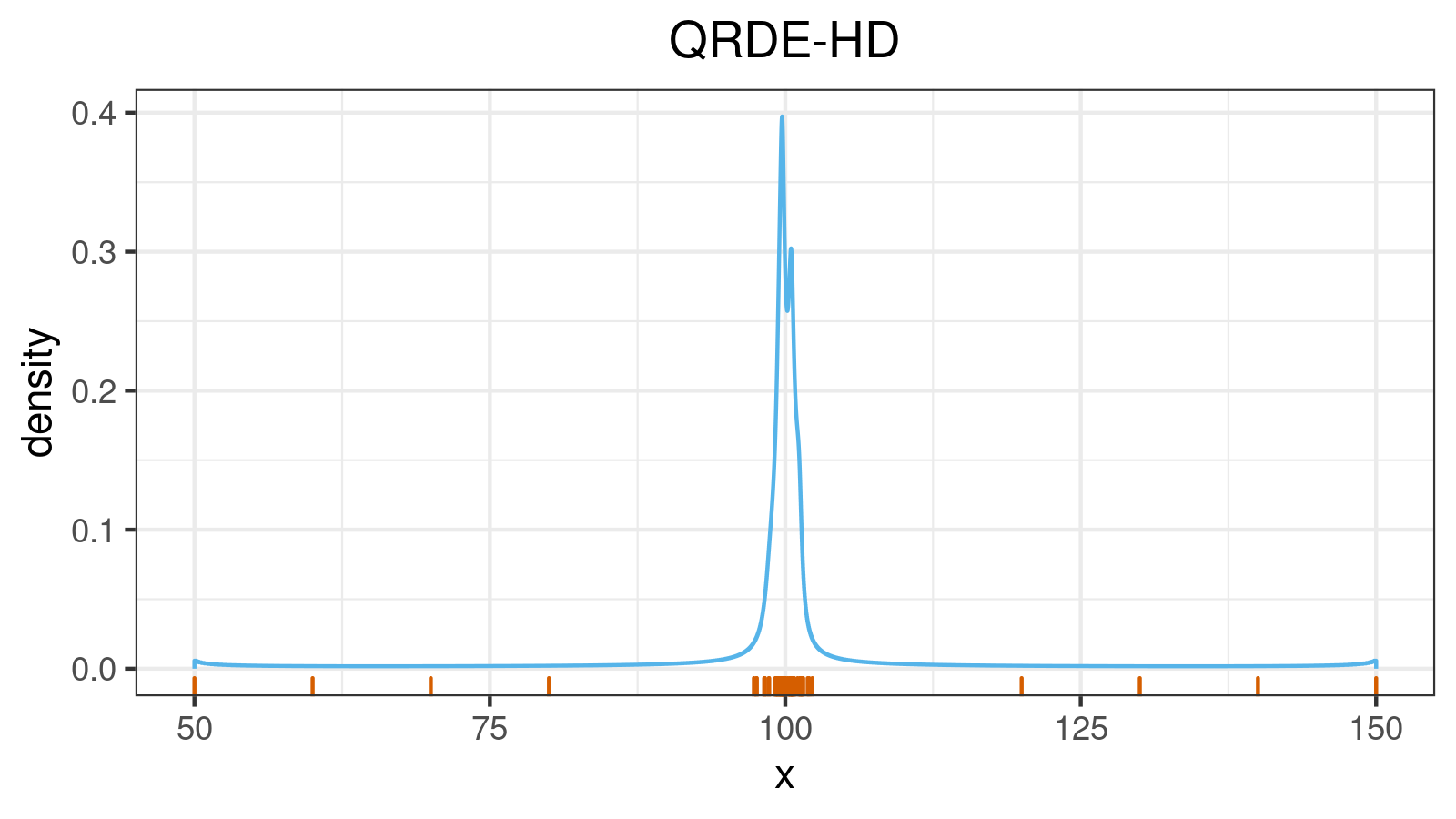
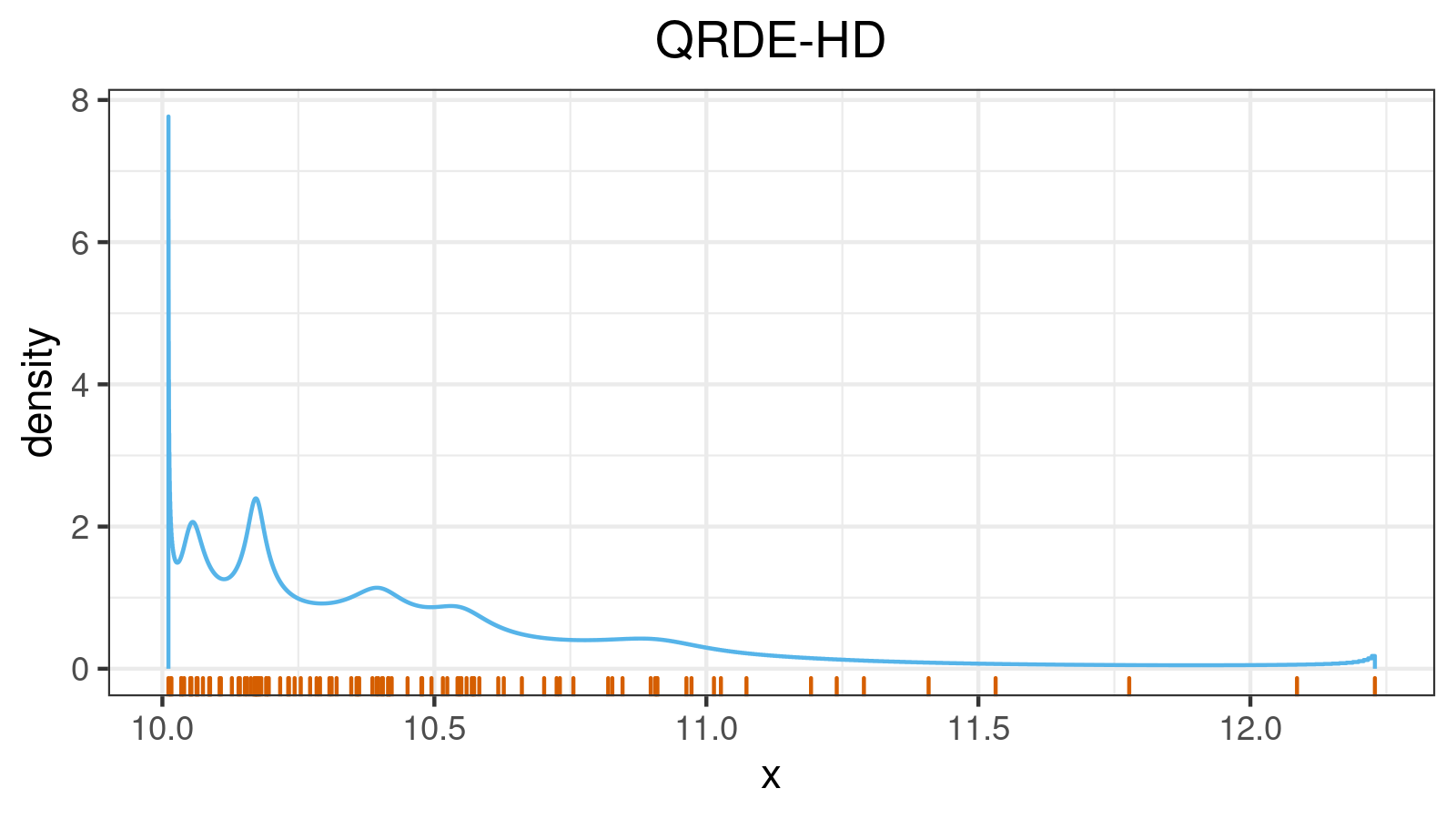
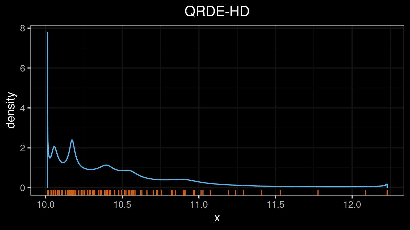
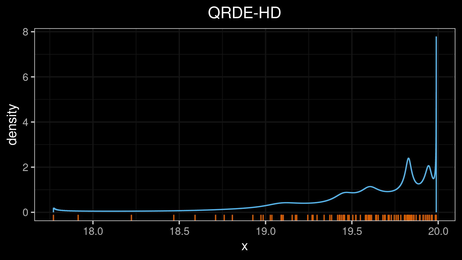
That’s how it looks for the unimodal case (the density plot is shown using the quantile-respectful density estimation based on the Harrell-Davis quantile estimator (QRDE-HD)):


You may notice that the deviation for the lower and upper quantiles are much larger than the deviation for the median. It’s a nice feature of this metric because it correlates with the estimator errors. Indeed, it’s hard to estimate extreme quantiles with high accuracy, and the errors are usually pretty large.
Now let’s add a few outliers and check out the updated $\mathcal{MAD}(x, p)$ plot:


We can see that the deviation for the extreme upper quantiles is much larger than the other $\mathcal{MAD}(x, p)$ values. It’s also an expected effect: when we have a few upper outliers, it’s tough to estimate the upper quantiles.
We have a similar situation for skewed distributions:


Quantile absolute deviation around quantiles
Now it’s time to make the final step toward generalizations. In the previous section, we took the median of $|x_i - Q(x, p)|$ to describe the dispersion around the given quantile. Can we estimate another quantile of $|x_i - Q(x, p)|$ instead of the median? Of course, we can! Let’s introduce the quantile absolute deviation around the given quantile:
$$ \mathcal{QAD}(x, p, q) = C \cdot Q(|x_i - Q(x, p)|, q). $$In the equation, we take $q^{\textrm{th}}$ quantile of $|x_i - Q(x, p)|$. This value also describes the dispersion around the $p^{\textrm{th}}$ quantile of $x$ similar to $\mathcal{MAD}(x, p)$, but it captures another interval of the distribution. To be more specific, $[Q(x, p) - \mathcal{QAD}(x, p, q); Q(x, p) + \mathcal{QAD}(x, p, q)]$ contains $(q*100)\%$ of the whole distribution.
The $\mathcal{QAD}$ is especially useful when we work with multimodal distribution. Let’s look at $\mathcal{QAD}(x, p, q)$ for $q \in {0.25, 0.5, 0.75}$ in the bimodal case:


Here we can see that the median absolute deviation around the median ($\mathcal{MAD}(x, 0.5) = \mathcal{QAD}(x, 0.5, 0.5)$) is much lower than the median absolute deviation around lower and upper quantiles (corner points of the $\mathcal{QAD}(x, p, 0.5)$ plot). It’s doesn’t actually meet our expectations. Indeed, the perfectly bimodal distribution is the worst case for the median estimation. Classic quantile estimators based on linear interpolation are incapable of estimating the median correctly because there are no sample elements around the true median value. The Harrell-Davis quantile estimator solves this problem much better, but the accuracy level is still low. Thus, we may expect that the deviation around the median (and the estimation errors) should be high. These expectation may be satisfied using $\mathcal{QAD}(x, 0.5, 0.25)$ which has the global maximum that matches the median.
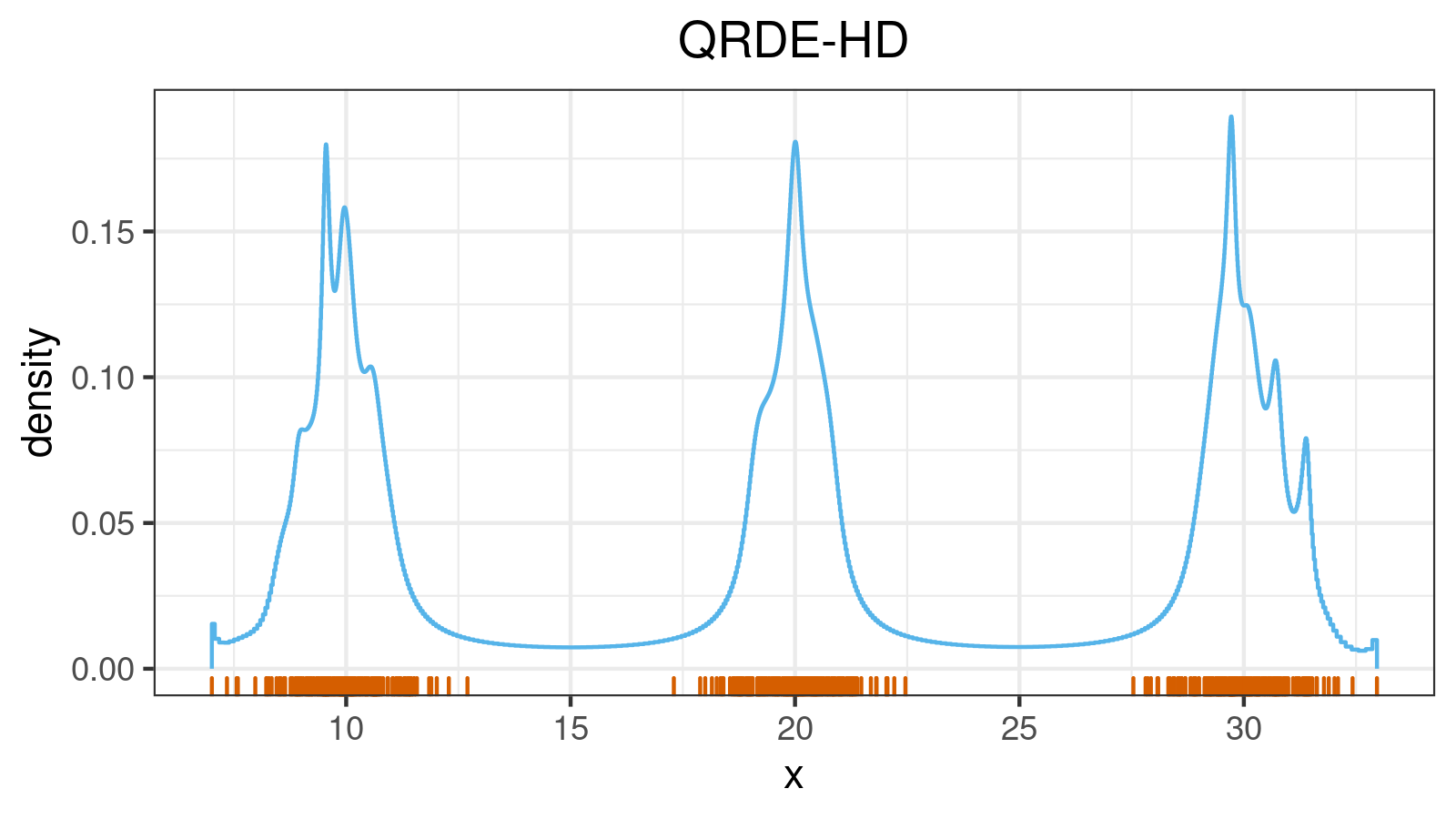
On the other hand, $\mathcal{QAD}(x, p, 0.75)$ is also may be useful. It captures 75% of the distribution, so it has a higher value at the mode values. We can see that $\mathcal{QAD}(x, 0.25, 0.75)$ is much larger than $\mathcal{QAD}(x, 0.5, 0.75)$. Thus, $\mathcal{QAD}(x, p, 0.75)$ is trying to say that the distance from the first mode to another one is larger than the distance from the median to the nearest mode. Using the $\mathcal{QAD}(x, p, q)$ plots for different $q$ values, we can get different insights about the distribution properties. Try to do it yourself with the trimodal distribution:


Of course, it’s not very convenient to manually enumerate different values of $q$ and look at dozens of plots. We need one more way to visualize the quantile absolute deviation to discover its true power.
Heatmap for Quantile absolute deviation around quantiles
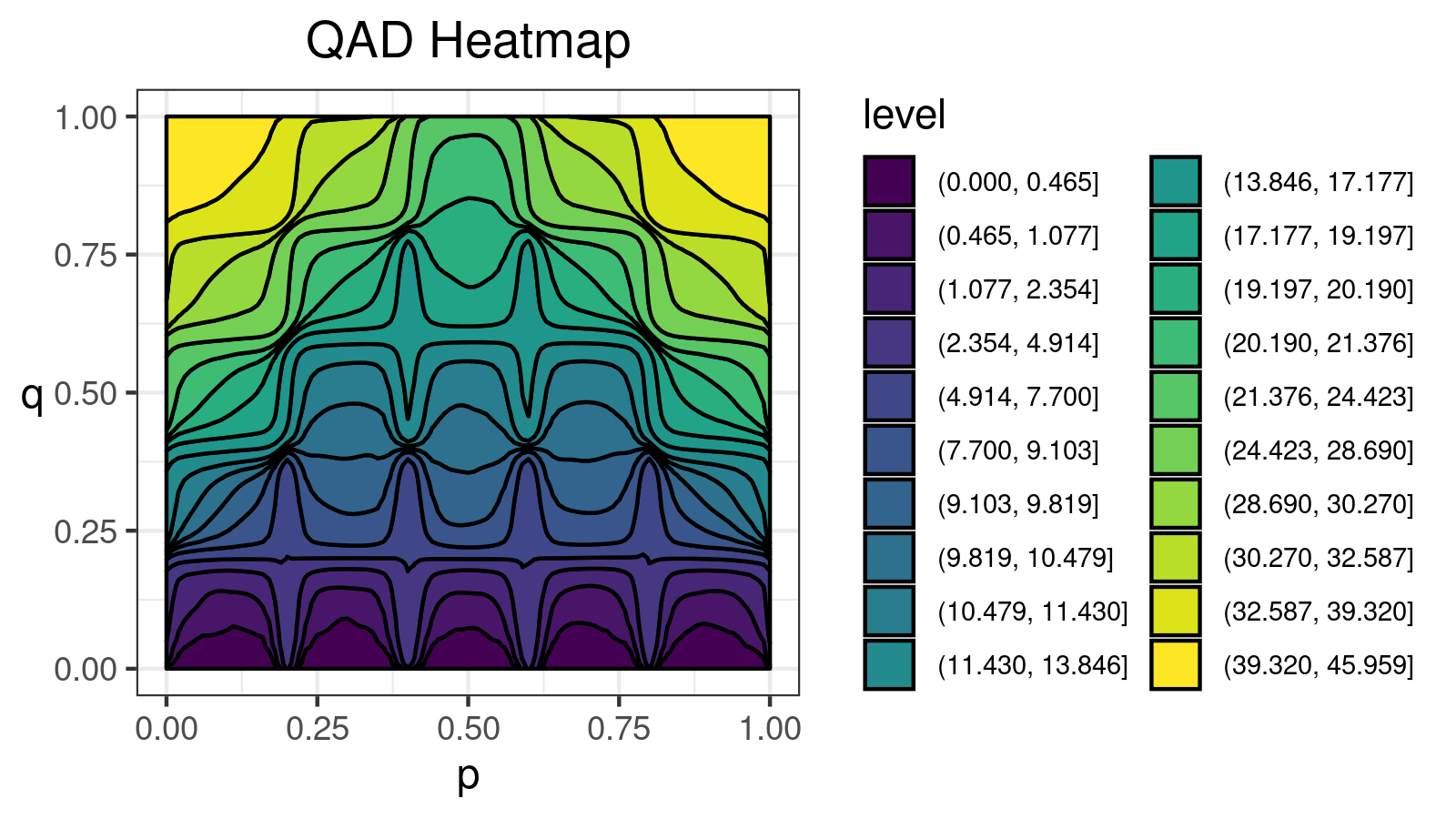
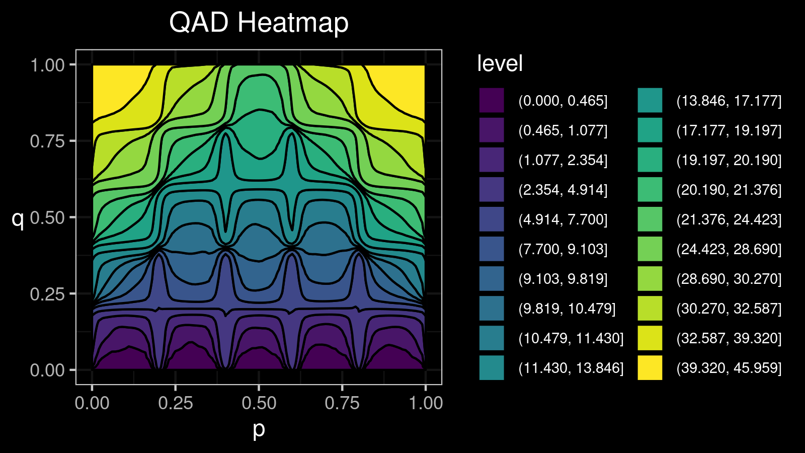
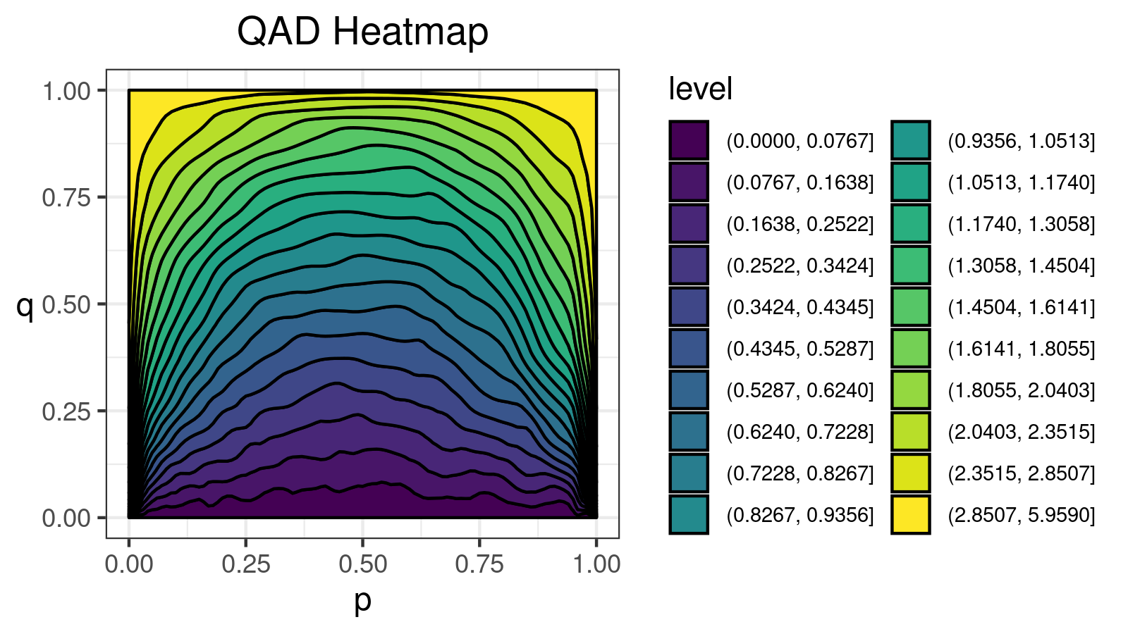
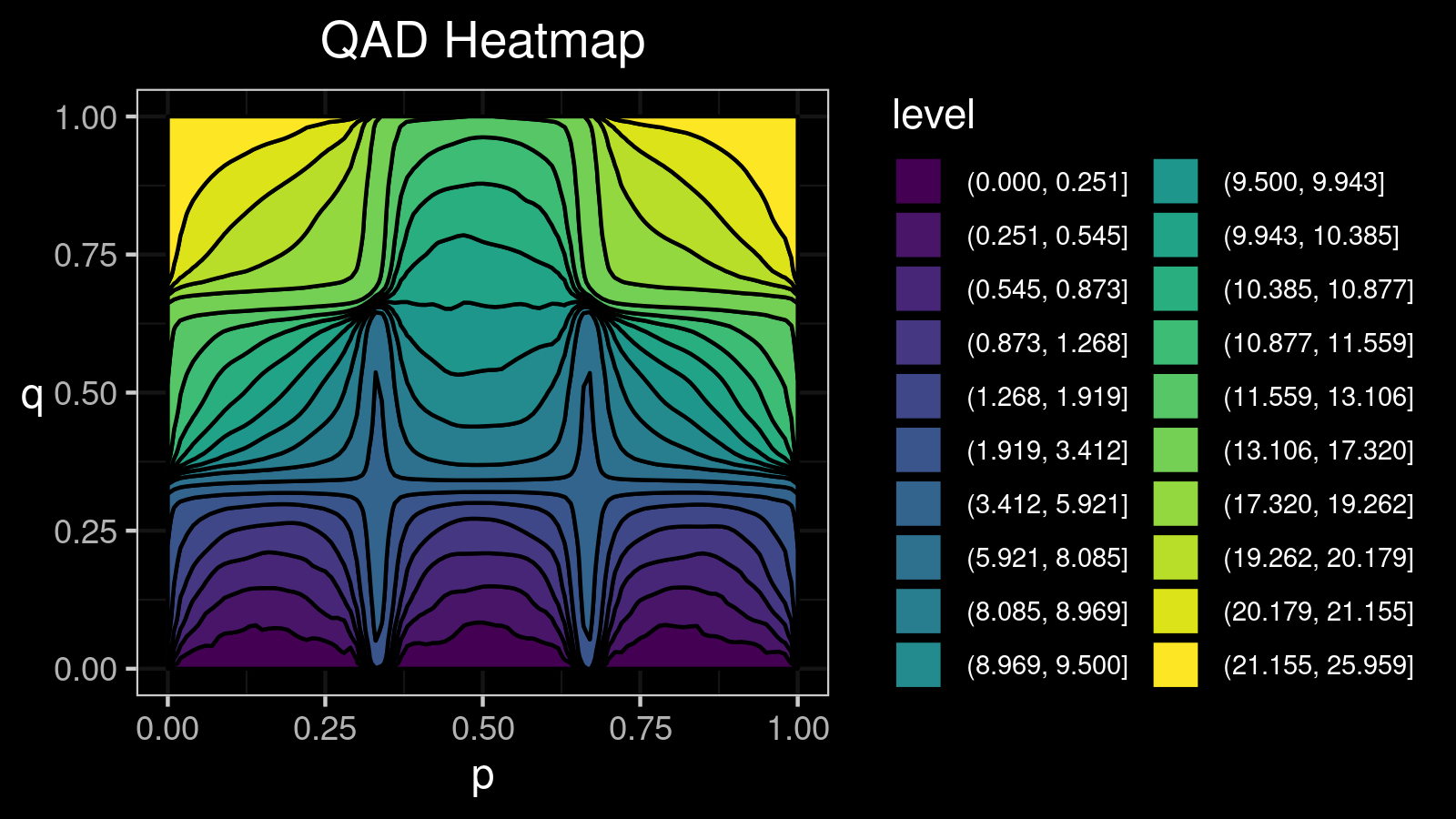
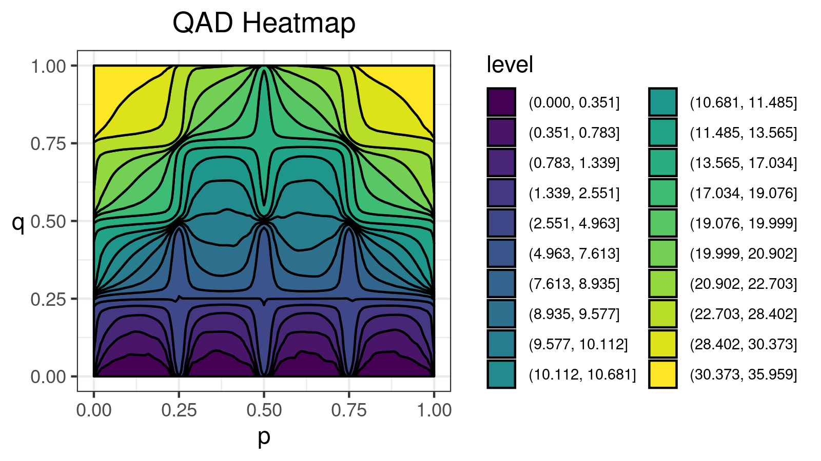
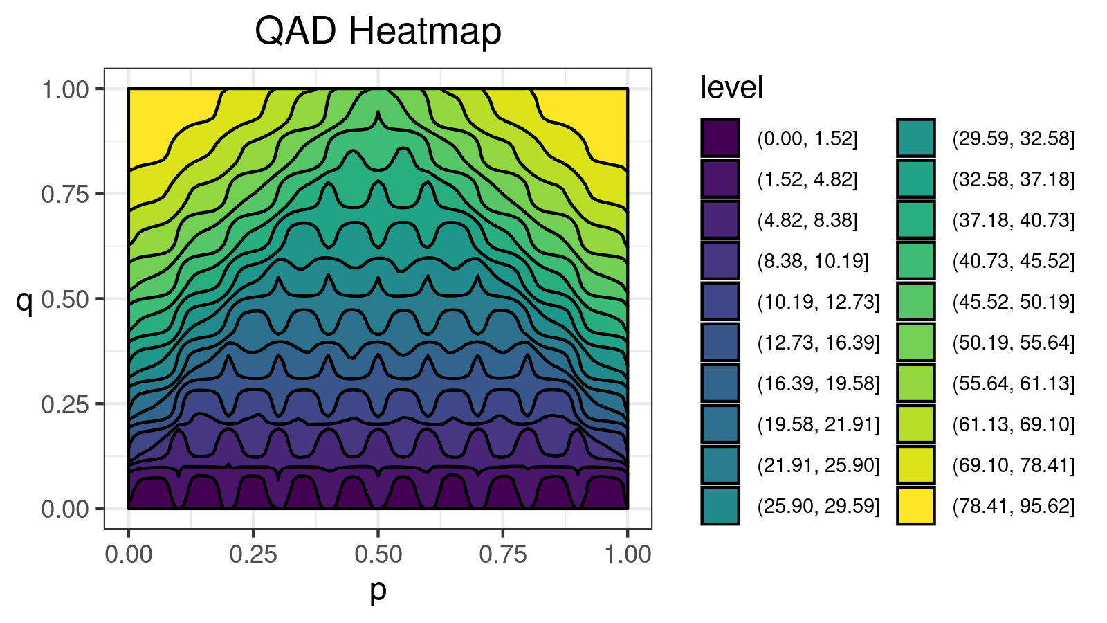
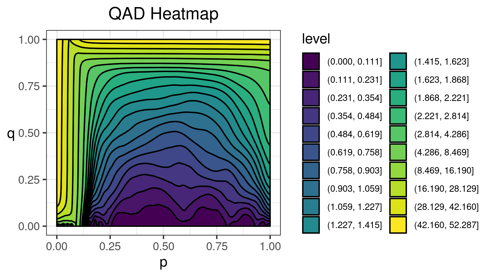
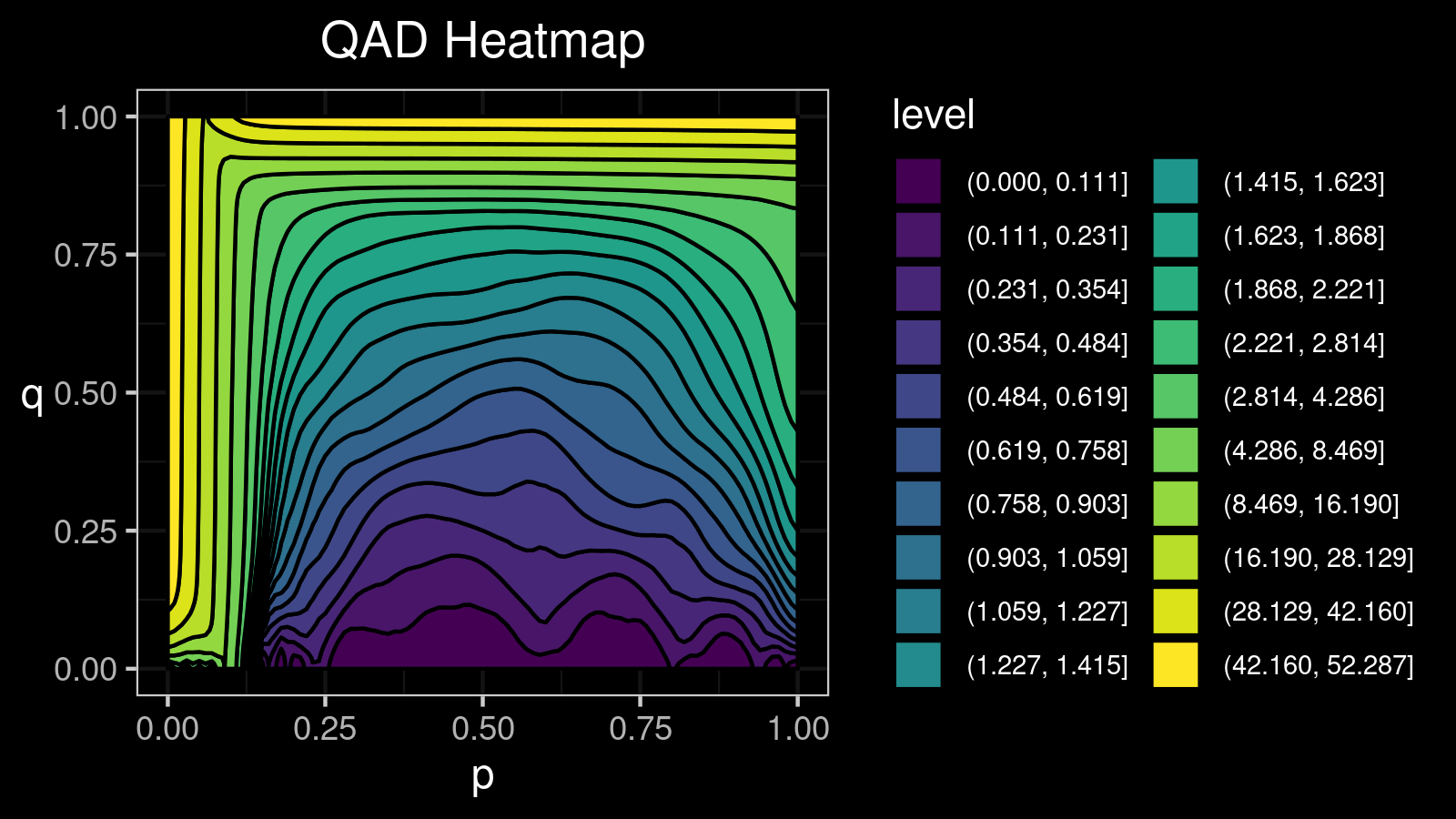
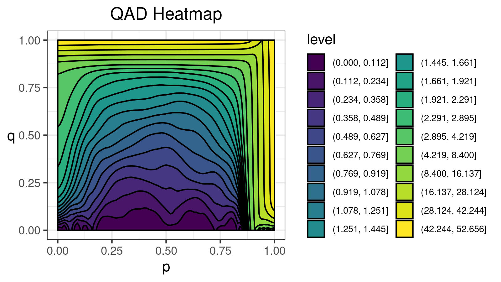
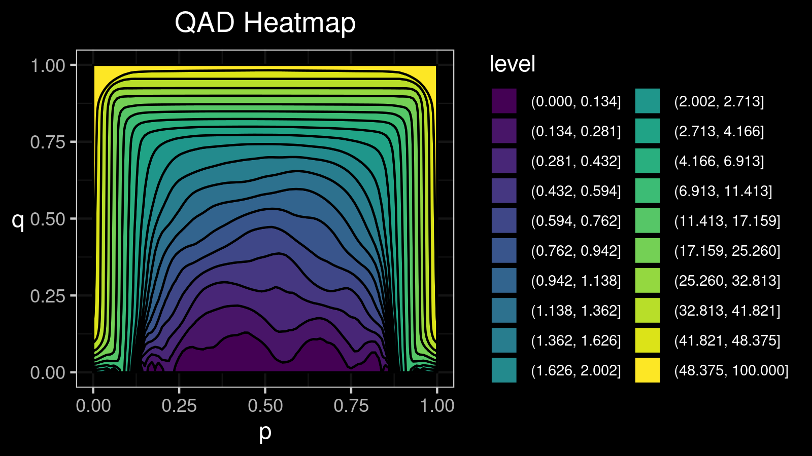
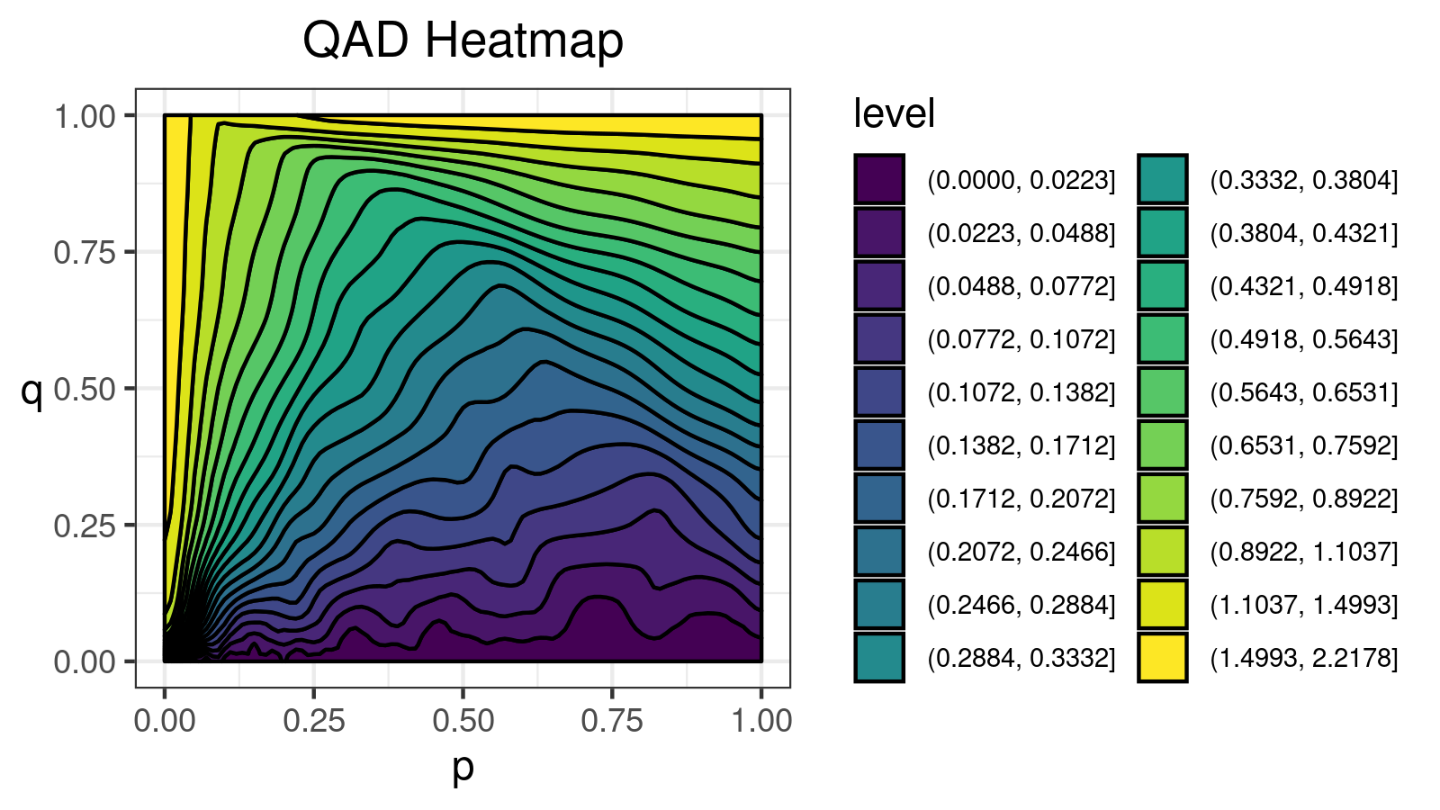
For the given $x$, $\mathcal{QAD}(x, p, q)$ is a function parameterized by two variables $p, q \in [0; 1]$. One of the most popular ways to visualize such functions is the heatmap. It’s also convenient to introduce several levels on this heatmap to highlight regions with the same value. I did a lot of experiments and came to the conclusion that I get the most insightful pictures using 20 levels. To split the whole range of $\mathcal{QAD}$ values to sub-intervals, we can use ventiles (20-quantiles). To get the ventile values, we use the Harrell-Davis quantile estimator one more time to get a smoother picture.
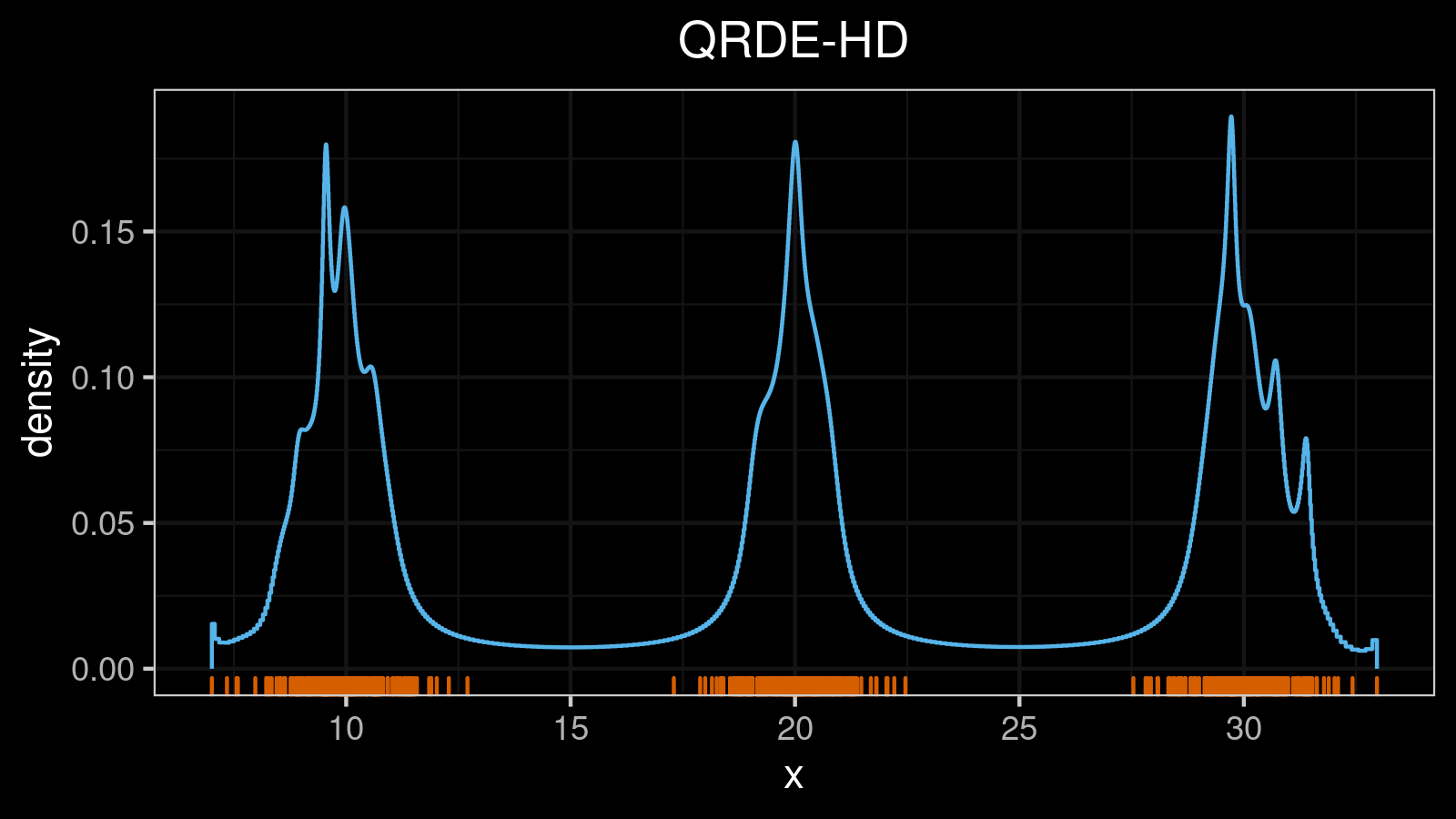
Consider a bimodal distribution:
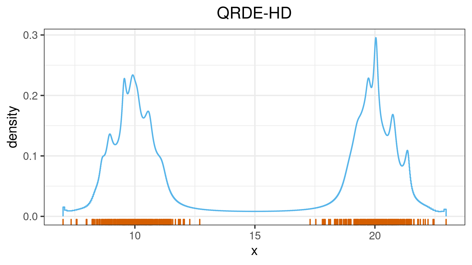
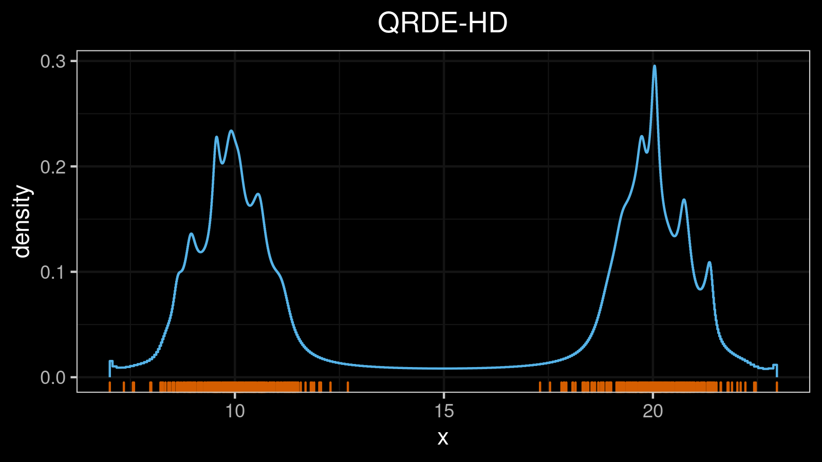
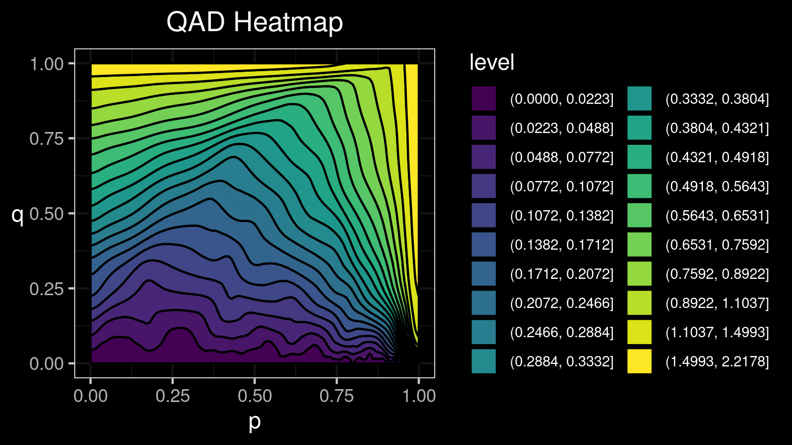
For this distribution, we get the following $\mathcal{QAD}$ heatmap:
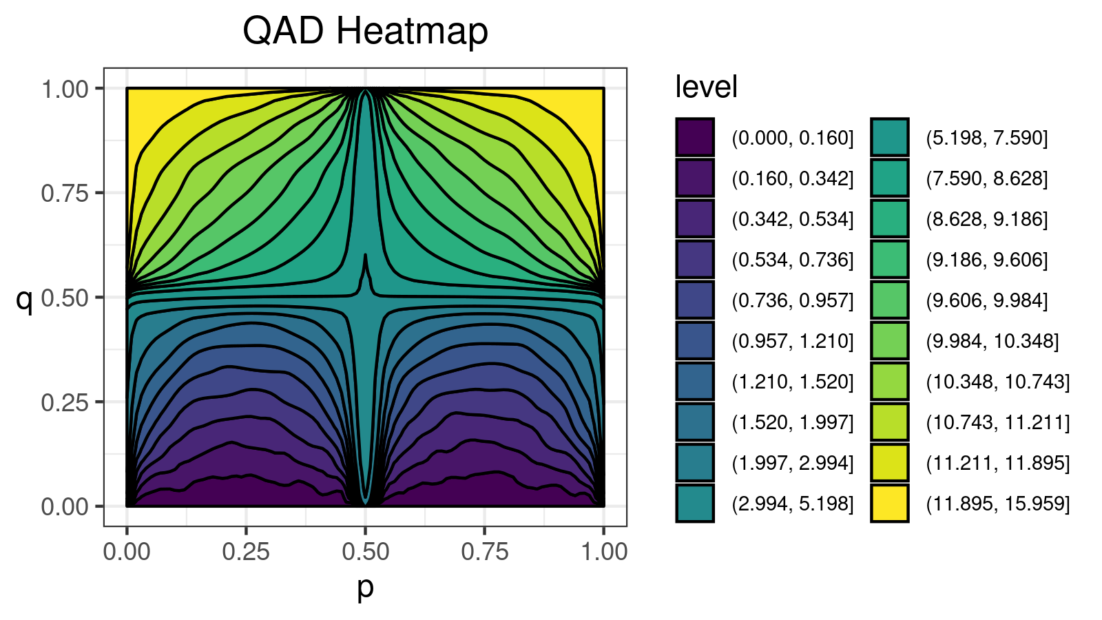
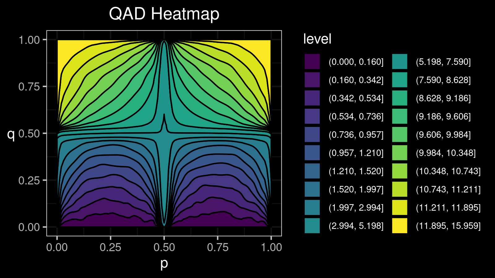
I made a lot of attempts trying to explain in the text form how to interpret such pictures. Unfortunately, I failed. I just don’t know how to express its internal beauty and the insightfulness of all the small details.
If you want to learn how to get benefits from such a visualization, just try to look at the different $\mathcal{QAD}$ heatmaps for a while and match them with the corresponding density plots. It should train the neural network inside your brain to work with these pictures. Below you find a gallery of such heatmaps for different distributions.
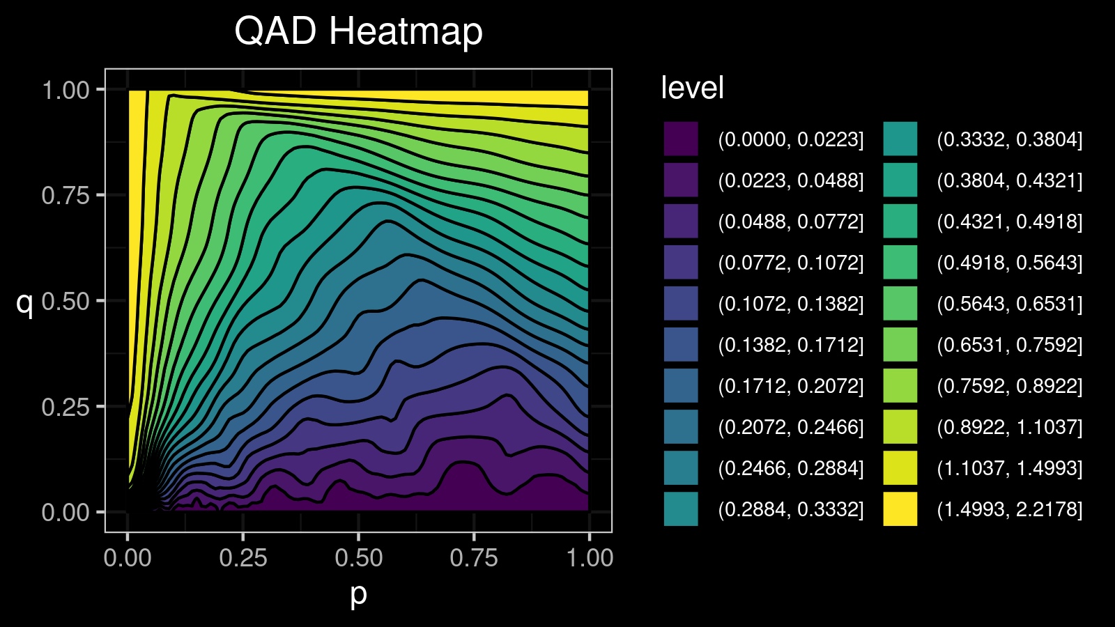
Heatmap gallery
A distribution with 1 mode:

A distribution with 2 modes:
A distribution with 3 modes:

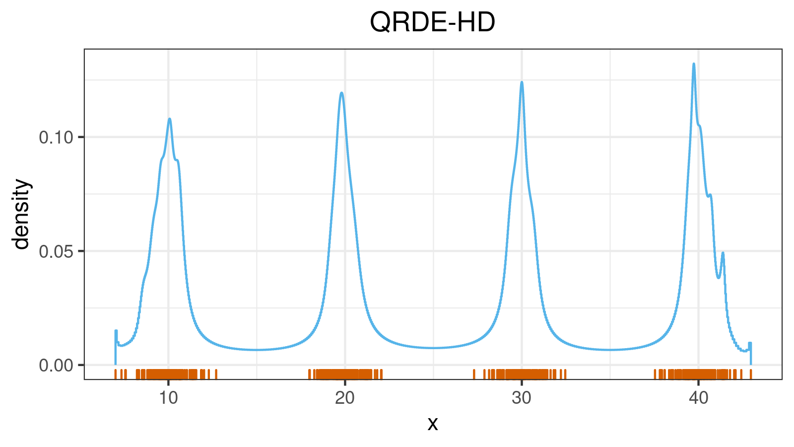
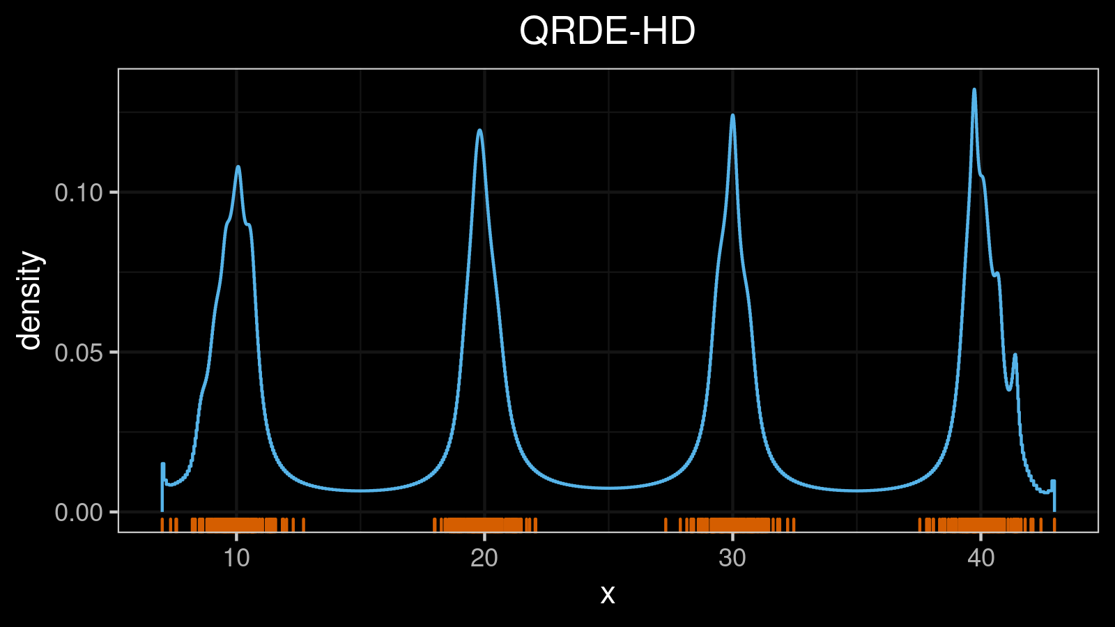
A distribution with 4 modes:

A distribution with 5 modes:
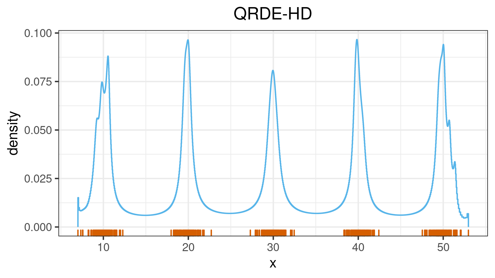
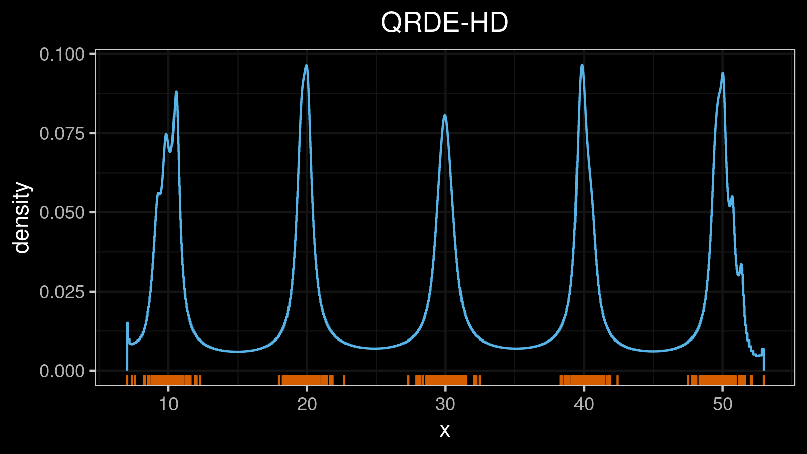
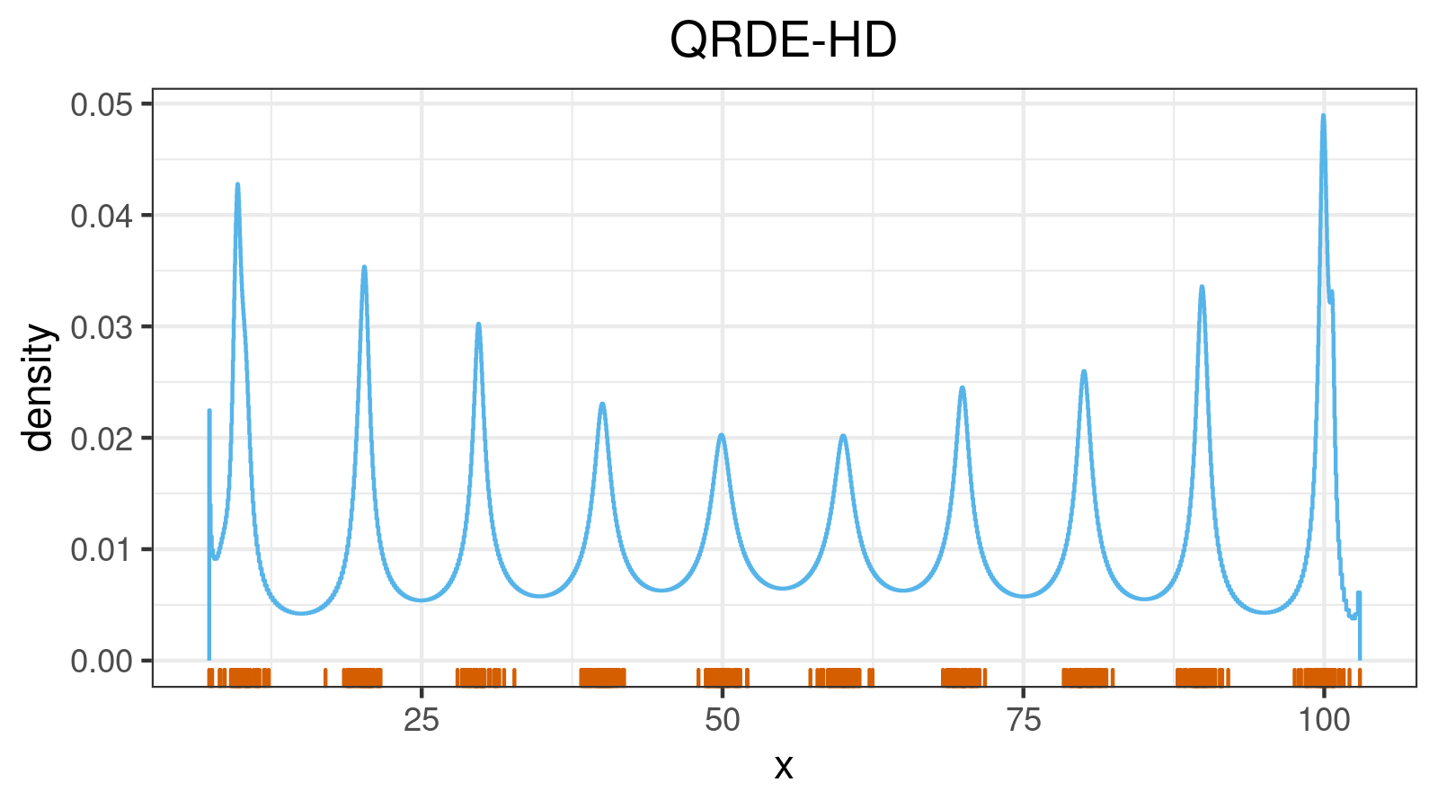
A distribution with 10 modes:

A distribution with lower outliers:
A distribution with upper outliers:
A distribution with lower and upper outliers:

A right-skewed distribution:

A left-skewed distribution:

Conclusion
In this post, I showed how to generalize the median absolute deviation ($\mathcal{MAD}$) around the median to the quantile absolute deviation ($\mathcal{QAD}$) around the given quantile. We discussed a few kinds of insightful visualization that may help you understand the nature of this metric.
I believe that the $\mathcal{QAD}$ is a powerful way to describe the statistical dispersion around the given quantile. In future blog posts, I will show how to use it to describe the overall distribution properties and how to use it to determine the quantile estimation errors.
References
- [Harrell1982]
Harrell, F.E. and Davis, C.E., 1982. A new distribution-free quantile estimator. Biometrika, 69(3), pp.635-640.
https://pdfs.semanticscholar.org/1a48/9bb74293753023c5bb6bff8e41e8fe68060f.pdf